Usage Note 70813: Produce heatmap of correlations, distances, differences, odds or hazard ratios, p-values or matrices of other numeric statistics
 |  |  |
A graphic depicting the values in a numeric matrix of any sort can be created using the HEATMAPPARM statement in PROC SGPLOT. The range of numeric values are represented using a color gradient with more extreme values shown using bolder, more saturated colors. In this way, extreme values stand out and clusters of similar values, appearing as regions of similar color, are more apparent than they are in a display of a purely numeric matrix.
The interpretation and understanding of many types of numeric matrices can be enhanced by the use of a heatmap representation. For example, a heatmap of a correlation matrix allows you to quickly see extreme values near the -1 or 1 limit. Similarly, with a distance matrix shown as a heatmap, the largest and smallest distances stand out with deeper colors and items with similar distances have similar colors. In a modeling context, a set of pairwise comparisons among levels of a CLASS variable, using mean differences, odds ratios, or hazard ratios, could be summarized with a heatmap. A companion heatmap can also be made of the p-values from those comparison statistics.
The first step in producing a heatmap from a numeric matrix is to arrange the data from a wide, square format into a long format in which all numeric values in the matrix appear in separate observations. This can be done in a DATA step. In some cases, such as data from the LSMEANS/DIFF statement, the necessary data is already in this long format. Also, if the values to be represented by a color range are from a bounded statistic, such as a correlation or p-value, and if you want the colors to be most extreme at the known bounds of the statistic rather than at the observed extremes, then observations containing the known statistic bounds should be added.
This note provides examples of producing heatmaps for correlation matrices and mean differences. Similar code can be used to display heatmaps for distances, odds or hazard ratios, relative risks, marginal effects, or essentially any other numeric matrix.
Heatmaps of Correlations and p-values
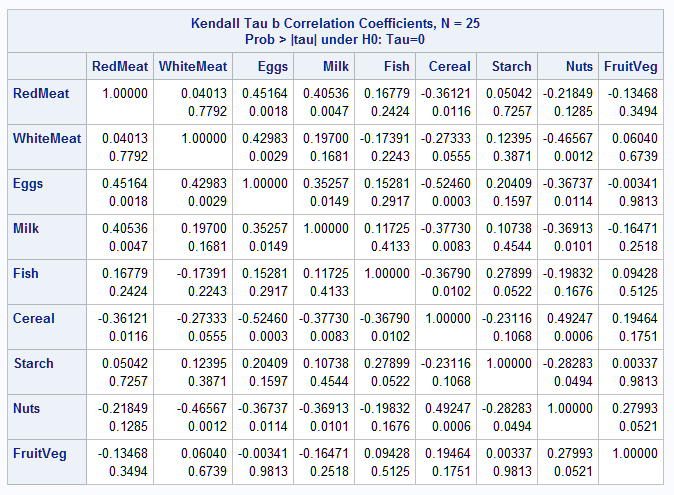
The following example uses the protein data in the Getting Started section of the DISTANCE procedure documentation in the SAS/STAT® User's Guide. The matrix of Kendall correlations among all numeric variables is produced by PROC CORR and is saved in data set CORRS using an ODS OUTPUT statement:
   proc corr data=protein kendall;
      var _numeric_;
      ods output kendallcorr=corrs;
      run;
Below is the numeric matrix produced by the procedure showing both the correlation values and p-values. As you can see, the extreme correlations, or patterns among them, do not stand out visually with this numerical matrix:
 |
Note the form of the correlation matrix and p-values saved in data set CORRS:
 |
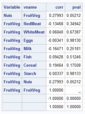
The following DATA step transforms the CORRS data set from a wide to a long format. Since all p-value variables begin with the letter P and none of the original variables begin with P, the set of p-value variables for the P array can be abbreviated p:. The VNAME function returns the name of the i-th variable in the C array. The last few lines add two observations that contain the bounding values of the correlation statistic (-1 and 1) and p-value (0 and 1). The variable names associated with them are assigned null values so that they do not form an additional block in the graphic:
   data long; set corrs end=eof;
      keep variable vname corr pval;
      array c (*) RedMeat WhiteMeat Eggs Milk Fish Cereal Starch Nuts FruitVeg;
      array p (*) p:;
      do i=1 to dim(c);
         vname=vname(c(i));
         corr=c(i); pval=p(i);
         output;
      end;
      if eof then do;
         variable=''; vname=''; corr=-1; pval=0; output;
         variable=''; vname=''; corr=1; pval=1; output;
      end;
      run;
The last few observations in the LONG data set are displayed below:
 |
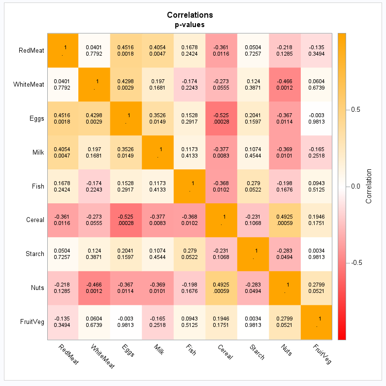
In the following, the HEATMAPPARM statement produces the heatmap of the correlation matrix using colors that represent the correlation values. The COLORMODEL= option uses the most saturated red for correlations near the -1 lower limit and the most saturated orange for correlations near the 1 upper limit. Correlations near zero appear white. TEXT statements are used to write the correlation value in each block with the associated p-value below. To properly display very small p-values (none occurring in this example), the FORMAT statement is used to assign the PVALUE format to the PVAL variable. The NOAUTOLEGEND option is used to suppress the unneeded legend below the graphic. Because this also suppresses the gradient bar, the GRADLEGEND statement is specified. The unneeded axis labels and tick marks are suppressed by the XAXIS and YAXIS statements. In order to preserve the row and column ordering of the correlation matrix, the REVERSE option is needed in the YAXIS statement. To prevent the text from overflowing the blocks or being too crowded, the HEIGHT= and WIDTH= options in the ODS GRAPHICS statement are specified to increase the size of the heatmap:
   ods graphics / height=8in width=8in;
   proc sgplot data=long noautolegend;
      heatmapparm x=variable y=vname colorresponse=corr / colormodel=(red white orange);
      text x=variable y=vname text=corr / position=top;
      text x=variable y=vname text=pval / position=bottom;
      gradlegend / title="Correlation";
      xaxis display=(nolabel noticks);
      yaxis reverse display=(nolabel noticks);
      format pval pvalue6.;
      title "Correlations";
      title2 "p-values";
      run;
With this depiction of the correlation matrix, the mostly negative correlations of cereal and nuts with the other variables stand out because their rows and columns are predominantly red. The block of more positive correlations among the meats, eggs, and milk also stands out:
 |
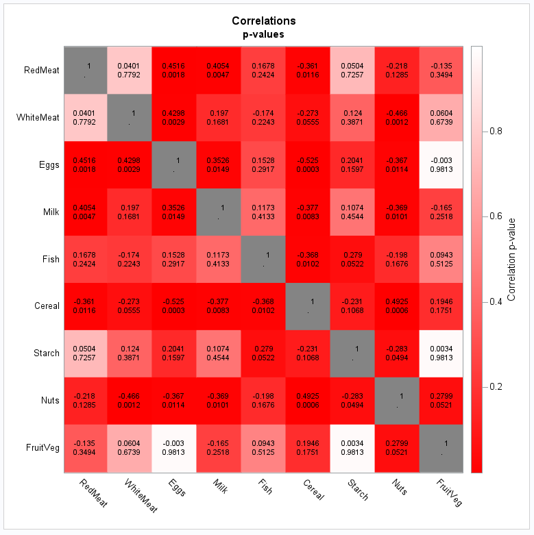
You might want to display the same matrix but instead color the blocks according to the p-value. The COLORMODEL= option now displays the most significant (smallest) p-values with the most saturated red and least significant (largest) p-values as white. Again, the FORMAT statement is used to assign the PVALUE format to the PVAL variable. Finally, the size options are reset to default values in the ODS GRAPHICS statement:
   proc sgplot data=long noautolegend;
      heatmapparm x=variable y=vname colorresponse=pval / colormodel=(red white);
      text x=variable y=vname text=corr / position=top;
      text x=variable y=vname text=pval / position=bottom;
      gradlegend / title="Correlation p-value";
      xaxis display=(nolabel noticks);
      yaxis reverse display=(nolabel noticks);
      format pval pvalue6.;
      title "Correlations";
      title2 "p-values";
      run;
   ods graphics / reset;
This coloration of the matrix makes it immediately clear that most correlations are pretty significant, whether positive or negative, as shown by the predominant appearance of red:
 |
Heatmap of a Correlation Matrix of Model Parameters
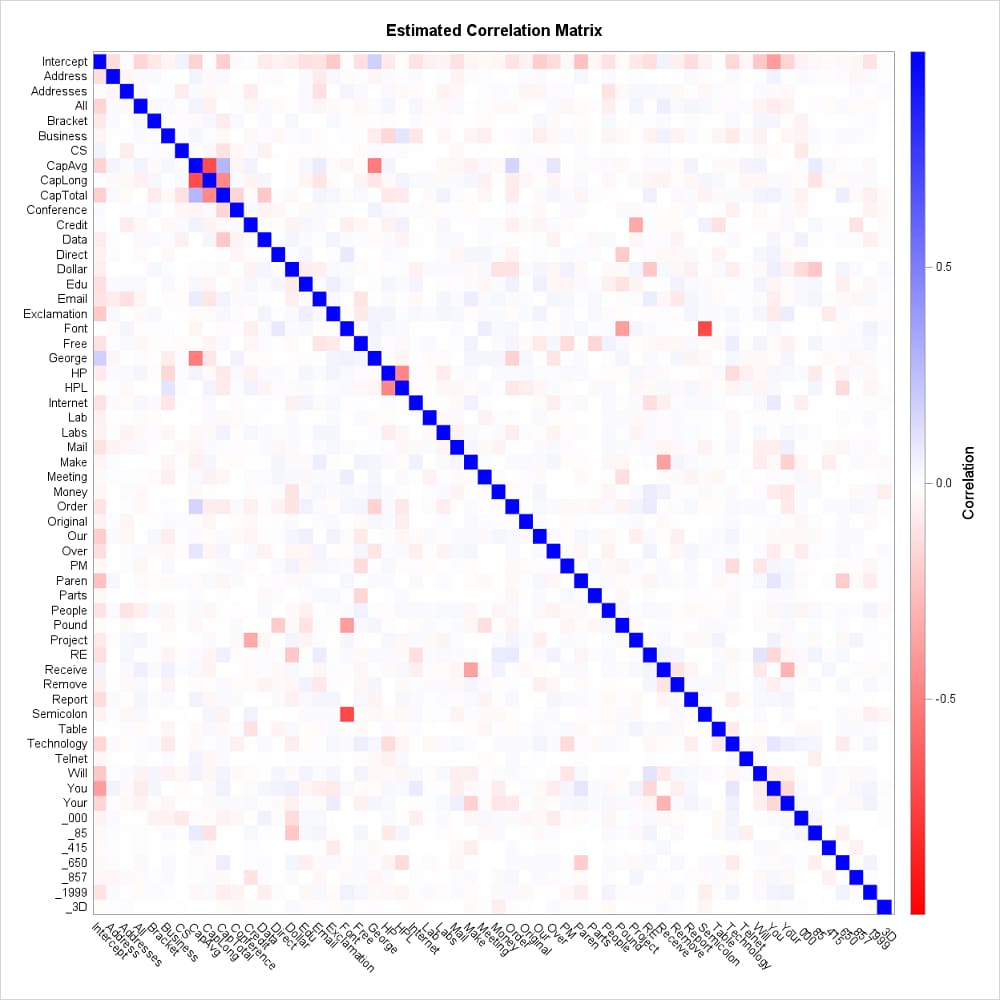
When the matrix contains a large number of entries, printing values within the individual blocks is not feasible. The following display of the correlation matrix of the parameters from a logistic model can assist in the assessment of collinearity, but it is not definitive of that condition as further discussed in SAS Note 32471.
Code similar to the above example produces the heatmap. The HEIGHT= and WIDTH= options in the ODS GRAPHICS statements specify a large enough graphic to allow for display of all variable names on both axes:
   ods exclude all;
   proc logistic data=sashelp.junkmail;
      model class(event='1') =
            Address     Addresses    All       Bracket    Business
            CS          CapAvg       CapLong   CapTotal   Conference
            Credit      Data         Direct    Dollar     Edu
            Email       Exclamation  Font      Free       George
            HP          HPL          Internet  Lab        Labs
            Mail        Make         Meeting   Money      Order
            Original    Our          Over      PM         Paren
            Parts       People       Pound     Project    RE
            Receive     Remove       Report    Semicolon  Table
            Technology  Telnet       Will      You        Your
            _000        _85          _415      _650       _857
            _1999       _3D / corrb;
      ods output corrb=corrb;
      run;
   ods select all;
   data long; set corrb end=eof;
      keep parameter vname corr;
      array v (*) _numeric_;
      do i=1 to dim(v);
         vname=vname(v(i));
         corr=v(i);
         output;
      end;
      if eof then do;
         parameter=''; vname=''; corr=-1; output;
         parameter=''; vname=''; corr=1; output;
      end;
      run;
   ods graphics / height=13in width=13in;
   proc sgplot data=long noautolegend;
      heatmapparm x=parameter y=vname colorresponse=corr / colormodel=(red white blue);
      gradlegend / title="Correlation";
      xaxis display=(nolabel noticks);
      yaxis reverse display=(nolabel noticks);
      title "Estimated Correlation Matrix";
      run;
   ods graphics / reset;
The few stronger correlations, such as between Semicolon and Font, stand out:
 |
Heatmap of Mean Comparisons Using LSMEANS
Producing a heatmap of mean comparisons can be simplified when using the LSMEANS statement. The data set that can be created from the differences table (DIFF option) is in a format that can be used directly with the HEATMAPPARM statement in PROC SGPLOT. But limit observations can be added if color range control is desired.
The following statements estimate the means of the Type levels and save the table of mean differences from the DIFF option in data set DIFFS:
   data plants;
      input Type $ @;
      do Block = 1 to 3;
         input StemLength @;
         output;
      end;
      datalines;
   Clarion  32.7 32.3 31.5
   Clinton  32.1 29.7 29.1
   Knox     35.7 35.9 33.1
   O'Neill  36.0 34.2 31.2
   Compost  31.8 28.0 29.2
   Wabash   38.2 37.8 31.9
   Webster  32.5 31.1 29.7
   ;
   proc glimmix data=plants;
      class Block Type;
      model StemLength = Block Type;
      lsmeans type / diff;
      ods output diffs=diffs;
      run;
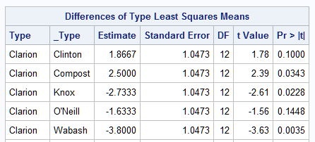
The first five mean comparisons in data set DIFFS are shown below. Notice that the data set is structured with one difference per observation rather than as a square matrix. In this form, the X=, Y=, and COLORRESPONSE= variables are available for use in SGPLOT directly:
 |
However, if you want to control the color range in the heatmap, for the differences or the p-values, then you can add limiting values with a DATA step as done in the examples above. To require that a difference of zero maps to the middle color in the range (white, in the following), find the most extreme mean difference (positive or negative) and add observations with positive and negative values of that extreme. The following statements add observations with those limits for the mean differences and limits, as above, for the p-values. Then, SGPLOT produces the heatmap of the mean differences using a suitable size:
   proc summary data=diffs;
      var estimate;
      output out=xtrem min=min max=max;
      run;
   data diffs; set diffs end=eof;
      output;
      if eof then do;
         set xtrem;
         type=''; _type=''; estimate=-max(abs(min),abs(max)); probt=0; output;
         type=''; _type=''; estimate=max(abs(min),abs(max)); probt=1; output;
      end;
      run;
   ods graphics / height=8in width=8in;
   proc sgplot data=diffs noautolegend;
      heatmapparm x=type y=_type colorresponse=estimate / colormodel=(red white orange);
      text x=type y=_type text=estimate / position=top;
      text x=type y=_type text=probt / position=bottom;
      gradlegend / title="Mean Difference";
      xaxis display=(nolabel noticks);
      yaxis reverse display=(nolabel noticks);
      format probt pvalue6.;
      title "Mean Differences";
      title2 "p-values";
      run;
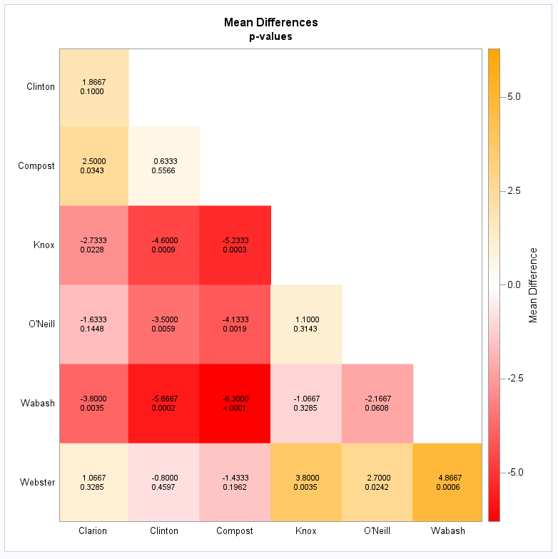
The colors in the heatmap distinguish the positive and negative differences with larger differences using the most saturated colors and small differences being closer to white:
 |
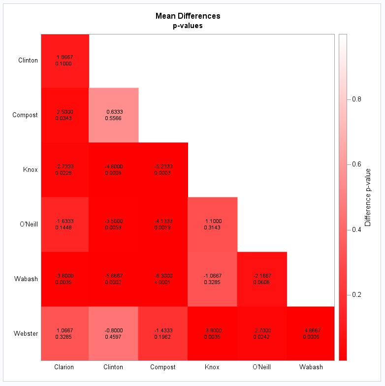
Similar code as before produces the heatmap colored by the p-values:
   proc sgplot data=diffs noautolegend;
      heatmapparm x=type y=_type colorresponse=probt / colormodel=(red white);
      text x=type y=_type text=estimate / position=top;
      text x=type y=_type text=probt / position=bottom;
      gradlegend / title="Difference p-value";
      xaxis display=(nolabel noticks);
      yaxis reverse display=(nolabel noticks);
      format probt pvalue6.;
      title "Mean Differences";
      title2 "p-values";
      run;
   ods graphics / reset;
The strong red saturation makes it clear that most differences are significant:
 |
Operating System and Release Information
| Product Family | Product | System | SAS Release | |
| Reported | Fixed* | |||
| SAS System | N/A | Windows 7 Enterprise 32 bit | ||
| Microsoft Windows Server 2022 | ||||
| Microsoft Windows XP Professional | ||||
| Microsoft Windows Server 2019 | ||||
| Microsoft Windows Server 2012 Std | ||||
| Microsoft Windows Server 2016 | ||||
| Microsoft Windows Server 2012 Datacenter | ||||
| Microsoft Windows Server 2008 for x64 | ||||
| Microsoft Windows Server 2003 for x64 | ||||
| Microsoft Windows Server 2008 | ||||
| OpenVMS Alpha | ||||
| Aster Data nCluster on Linux x64 | ||||
| DB2 Universal Database on AIX | ||||
| DB2 Universal Database on Linux x64 | ||||
| Netezza TwinFin 32-bit SMP Hosts | ||||
| Netezza TwinFin 32bit blade | ||||
| Netezza TwinFin 64-bit S-Blades | ||||
| Netezza TwinFin 64-bit SMP Hosts | ||||
| Teradata on Linux | ||||
| Cloud Foundry | ||||
| 64-bit Enabled AIX | ||||
| 64-bit Enabled HP-UX | ||||
| 64-bit Enabled Solaris | ||||
| ABI+ for Intel Architecture | ||||
| AIX | ||||
| HP-UX | ||||
| HP-UX IPF | ||||
| IRIX | ||||
| Linux | ||||
| Linux for AArch64 | ||||
| Linux for x64 | ||||
| Linux on Itanium | ||||
| Windows 7 Ultimate x64 | ||||
| Windows 7 Professional x64 | ||||
| Windows 7 Ultimate 32 bit | ||||
| Windows 7 Professional 32 bit | ||||
| Windows 7 Home Premium 32 bit | ||||
| Windows 7 Home Premium x64 | ||||
| Windows 7 Enterprise x64 | ||||
| Windows Vista for x64 | ||||
| Windows Vista | ||||
| Windows Millennium Edition (Me) | ||||
| OpenVMS on HP Integrity | ||||
| Solaris | ||||
| Solaris for x64 | ||||
| Tru64 UNIX | ||||
| z/OS | ||||
| z/OS 64-bit | ||||
| IBM AS/400 | ||||
| OpenVMS VAX | ||||
| N/A | ||||
| Android Operating System | ||||
| Apple Mobile Operating System | ||||
| Chrome Web Browser | ||||
| Macintosh | ||||
| Macintosh on x64 | ||||
| Microsoft Windows 10 | ||||
| Microsoft Windows 7 | ||||
| Microsoft Windows 8 Enterprise 32-bit | ||||
| Microsoft Windows 8 Enterprise x64 | ||||
| Microsoft Windows 8 Pro 32-bit | ||||
| Microsoft Windows 8 Pro x64 | ||||
| Microsoft Windows 8 x64 | ||||
| Microsoft Windows Server 2008 R2 | ||||
| Microsoft Windows Server 2012 R2 Datacenter | ||||
| Microsoft Windows Server 2012 R2 Std | ||||
| Microsoft® Windows® for 64-Bit Itanium-based Systems | ||||
| Microsoft Windows Server 2003 Datacenter 64-bit Edition | ||||
| Microsoft Windows Server 2003 Enterprise 64-bit Edition | ||||
| Microsoft Windows XP 64-bit Edition | ||||
| Microsoft® Windows® for x64 | ||||
| OS/2 | ||||
| SAS Cloud | ||||
| Microsoft Windows 8.1 Enterprise 32-bit | ||||
| Microsoft Windows 8.1 Enterprise x64 | ||||
| Microsoft Windows 8.1 Pro 32-bit | ||||
| Microsoft Windows 8.1 Pro x64 | ||||
| Microsoft Windows 11 | ||||
| Microsoft Windows 95/98 | ||||
| Microsoft Windows 2000 Advanced Server | ||||
| Microsoft Windows 2000 Datacenter Server | ||||
| Microsoft Windows 2000 Server | ||||
| Microsoft Windows 2000 Professional | ||||
| Microsoft Windows NT Workstation | ||||
| Microsoft Windows Server 2003 Datacenter Edition | ||||
| Microsoft Windows Server 2003 Enterprise Edition | ||||
| Microsoft Windows Server 2003 Standard Edition | ||||
| Type: | Usage Note |
| Priority: | |
| Topic: | Analytics ==> Statistical Graphics SAS Reference ==> Procedures ==> CORR SAS Reference ==> Procedures ==> DISTANCE SAS Reference ==> Procedures ==> SGPLOT |
| Date Modified: | 2024-06-04 10:05:45 |
| Date Created: | 2024-05-31 12:37:27 |