Sample 60848: A Simple Regression Model with Correction of Heteroscedasticity
 |  |  |  |
Overview
 |
One of the classical assumptions of the ordinary regression model is that the disturbance variance is constant, or homogeneous, across observations. If this assumption is violated, the errors are said to be "heteroscedastic." Heteroscedasticity often arises in the analysis of cross-sectional data. For example, in analyzing public school spending, certain states may have greater variation in expenditure than others. If heteroscedasticity is present and a regression of spending on per capita income by state and its square is computed, the parameter estimates are still consistent but they are no longer efficient. Thus, inferences from the standard errors are likely to be misleading.
Testing for Heteroscedasticity
There are several methods of testing for the presence of heteroscedasticity. The most commonly used is the Time-Honored Method of Inspection (THMI). This test involves looking for patterns in a plot of the residuals from a regression. Two more formal tests are White's General test (White 1980) and the Breusch-Pagan test (Breusch and Pagan 1979).
The White test is computed by finding nR2 from a regression of ei2 on all of the distinct variables in ![]() , where X is the vector of dependent variables including a constant. This statistic is asymptotically distributed as chi-square with k-1 degrees of freedom, where k is the number of regressors, excluding the constant term.
, where X is the vector of dependent variables including a constant. This statistic is asymptotically distributed as chi-square with k-1 degrees of freedom, where k is the number of regressors, excluding the constant term.
The Breusch-Pagan test is a Lagrange multiplier test of the hypothesis that the independent variables have no explanatory power on the ei2's. If u equals (e12, e22, . . . , en2), i equals an n ×1 column of ones, and ![]() , then Koenkar and Bassett's (1982) robust variance estimator
, then Koenkar and Bassett's (1982) robust variance estimator
computes the test statistic as
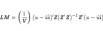
which is asymptotically distributed as chi-square with degrees of freedom equal to the number of variables in Z.
Correcting for Heteroscedasticity
One way to correct for heteroscedasticity is to compute the weighted least squares (WLS) estimator using an hypothesized specification for the variance. Often this specification is one of the regressors or its square.
This example uses the MODEL procedure to perform the preceding tests and the WLS correction in an investigation of public school spending in the United States.
Analysis
If y is public school spending and x is per capita income, and assuming that the variance of the error term is proportional to xi2, then the regression model in this example can be written as

where i = 1, ... ,51 is a state index.
The sample consists of 51 observations of per capita expenditure on public schools and per capita income for each state and the District of Columbia in 1979.
The following DATA step reads in the 51 observations, transforms the variable INC by multiplying it by 10-4 (for consistency with Greene 1993), creates the variable INC2 as the square of income, and then deletes Wisconsin from the sample due to a missing value for expenditure.
   data hetero1;
      input st exp inc;
         inc=inc/10000;
         inc2=inc**2;
      if exp = . then delete;
      datalines;
   1     275 6247
   2     275 6183
   3     531 8914
   ...
   ;
   run;
Testing for Heteroscedasticity
You can use the MODEL procedure for the initial investigation of the model. The following commands estimate the preceding model, perform two different tests for heteroscedasticity (the White and the Breusch-Pagan), and output the residuals into a data set for further investigation.
   proc model data=hetero1;
      parms a1 b1 b2;
      exp = a1 + b1 * inc + b2 * inc2;
      fit exp / white pagan=(1 inc inc2)
      out=resid1 outresid;
   run;
   quit;
The estimates for the constant term and the coefficients of INC and INC2 and their associated p-values are 832.91 (0.014), -1834.20 (0.032), and 1587.04 (0.004), respectively, which all appear to be different from 0 at generally accepted levels of statistical significance. Notice, however, that both the White test (21.16) and the Breusch-Pagan test (15.83) reject the null hypothesis of no heteroscedasticity. This implies that the standard errors of the parameter estimates are incorrect and, thus, any inferences derived from them may be misleading. A plot of the residuals shows more variance in the errors of higher income states.
Correcting for Heteroscedasticity
If the form of the variance is known, the WEIGHT= option can be specified in the MODEL procedure to correct for heteroscedasticity using weighted least squares (WLS). The following statement performs WLS using 1/(INC2) as the weight.
   proc model data=hetero1;
      parms a1 b1 b2;
      inc2_inv = 1/inc2;
      exp = a1 + b1 * inc + b2 * inc2;
      fit exp / white pagan=(1 inc inc2);
      weight inc2_inv;
   run;
   quit;
|
|||||||||||||||||||||||||||||||||||||||||||||||||||||||||||||||||||||||||||||||||||||||||||
The corrected estimates for the constant term and the coefficients of INC and INC2 and their associated p-values are 664.58 (0.052), -1399.28 (0.115), and 1311.35 (0.024), respectively. The significance of the estimates is greatly reduced, obscuring the individual effects of the explanatory variables. The White test (9.31) and the Breusch-Pagan test (5.23) are no longer significant at the 5% level.
All of the preceding calculations can be found in Greene (1993, chapter 14).
References
Breusch, T. and Pagan, A. (1979), ``A Simple Test for Heteroscedasticity and Random Coefficient Variation," Econometrica, 47, 1287-1294.
Greene, W.H. (1993), Econometric Analysis, Second Edition, New York: Macmillan Publishing Company.
Koenkar, R., and Basset, G. (1982), ``Robust Tests for Heteroscedasticity Based on Regression Quantiles," Econometrica, 50, 43-61.
SAS Institute Inc. (1993), SAS/ETS User's Guide, Version 6, Second Edition, Cary, NC: SAS Institute Inc.
White, H. (1980), ``A Heteroscedasticity-Consistent Covariance Matrix Estimator and a Direct Test for Heteroscedasticity," Econometrica, 48, 817-838.
These sample files and code examples are provided by SAS Institute Inc. "as is" without warranty of any kind, either express or implied, including but not limited to the implied warranties of merchantability and fitness for a particular purpose. Recipients acknowledge and agree that SAS Institute shall not be liable for any damages whatsoever arising out of their use of this material. In addition, SAS Institute will provide no support for the materials contained herein.
/* Regression Model with Correction of Heteroskedasticity */

data hetero1;
  input state exp inc;
   inc=inc/10000;
   inc2=inc**2;
  if exp = . then delete;
  datalines;
1     275 6247
2     275 6183
3     531 8914
4     316 7505
5     304 6813
6     431 7873
7     316 6640
8     427 8063
9     259 5736
10    294 7391
11    423 8818
12    335 6607
13    320 6951
14    342 7526
15    268 6489
16    353 6541
17    320 6456
18    821 10851
19    387 8850
20    424 8604
21    265 6700
22    437 8745
23    355 8001
24    327 6333
25    466 8442
26    274 7342
27    359 9032
28    388 6505
29    311 7478
30    397 7839
31    315 6242
32    315 7697
33    356 7624
34     .  7597
35    339 7374
36    452 8001
37    428 10022
38    403 8380
39    345 7696
40    260  6615
41    427  8306
42    477  7847
43    433  7051
44    279  7277
45    447  8267
46    322  7812
47    412  7733
48    321  6841
49    417  6622
50    415  8450
51    500  9096
;

/* Ordinary Least Squares */

title 'Ordinary Least Squares';

proc model data=hetero1;
  parms a1 b1 b2;
  exp = a1 + b1 * inc + b2 * inc2;
  fit exp / white pagan=(1 inc inc2)
  out=resid1 outresid;
run;
quit;

proc gplot data=resid1;
   plot exp*inc / vref=0 cvref=red;
   symbol c=blue value=star;
   title1 'Residual vs. Per Capita Income';
   title2 'Ordinary Least Squares';
run;
quit;

/* Weighted Least Squares */

title 'Weighted Least Squares';
title2;

proc model data=hetero1;
  parms a1 b1 b2;
  inc2_inv = 1/inc2;
  exp = a1 + b1 * inc + b2 * inc2;
  fit exp / white pagan=(1 inc inc2);
  weight inc2_inv;
run;
quit;
These sample files and code examples are provided by SAS Institute Inc. "as is" without warranty of any kind, either express or implied, including but not limited to the implied warranties of merchantability and fitness for a particular purpose. Recipients acknowledge and agree that SAS Institute shall not be liable for any damages whatsoever arising out of their use of this material. In addition, SAS Institute will provide no support for the materials contained herein.
| Type: | Sample |
| Date Modified: | 2017-07-31 15:24:17 |
| Date Created: | 2017-07-31 13:57:40 |
Operating System and Release Information
| Product Family | Product | Host | SAS Release | |
| Starting | Ending | |||
| SAS System | SAS/ETS | z/OS | ||
| z/OS 64-bit | ||||
| OpenVMS VAX | ||||
| Microsoft® Windows® for 64-Bit Itanium-based Systems | ||||
| Microsoft Windows Server 2003 Datacenter 64-bit Edition | ||||
| Microsoft Windows Server 2003 Enterprise 64-bit Edition | ||||
| Microsoft Windows XP 64-bit Edition | ||||
| Microsoft® Windows® for x64 | ||||
| OS/2 | ||||
| Microsoft Windows 8 Enterprise 32-bit | ||||
| Microsoft Windows 8 Enterprise x64 | ||||
| Microsoft Windows 8 Pro 32-bit | ||||
| Microsoft Windows 8 Pro x64 | ||||
| Microsoft Windows 8.1 Enterprise 32-bit | ||||
| Microsoft Windows 8.1 Enterprise x64 | ||||
| Microsoft Windows 8.1 Pro 32-bit | ||||
| Microsoft Windows 8.1 Pro x64 | ||||
| Microsoft Windows 10 | ||||
| Microsoft Windows 95/98 | ||||
| Microsoft Windows 2000 Advanced Server | ||||
| Microsoft Windows 2000 Datacenter Server | ||||
| Microsoft Windows 2000 Server | ||||
| Microsoft Windows 2000 Professional | ||||
| Microsoft Windows NT Workstation | ||||
| Microsoft Windows Server 2003 Datacenter Edition | ||||
| Microsoft Windows Server 2003 Enterprise Edition | ||||
| Microsoft Windows Server 2003 Standard Edition | ||||
| Microsoft Windows Server 2003 for x64 | ||||
| Microsoft Windows Server 2008 | ||||
| Microsoft Windows Server 2008 R2 | ||||
| Microsoft Windows Server 2008 for x64 | ||||
| Microsoft Windows Server 2012 Datacenter | ||||
| Microsoft Windows Server 2012 R2 Datacenter | ||||
| Microsoft Windows Server 2012 R2 Std | ||||
| Microsoft Windows Server 2012 Std | ||||
| Microsoft Windows XP Professional | ||||
| Windows 7 Enterprise 32 bit | ||||
| Windows 7 Enterprise x64 | ||||
| Windows 7 Home Premium 32 bit | ||||
| Windows 7 Home Premium x64 | ||||
| Windows 7 Professional 32 bit | ||||
| Windows 7 Professional x64 | ||||
| Windows 7 Ultimate 32 bit | ||||
| Windows 7 Ultimate x64 | ||||
| Windows Millennium Edition (Me) | ||||
| Windows Vista | ||||
| Windows Vista for x64 | ||||
| 64-bit Enabled AIX | ||||
| 64-bit Enabled HP-UX | ||||
| 64-bit Enabled Solaris | ||||
| ABI+ for Intel Architecture | ||||
| AIX | ||||
| HP-UX | ||||
| HP-UX IPF | ||||
| IRIX | ||||
| Linux | ||||
| Linux for x64 | ||||
| Linux on Itanium | ||||
| OpenVMS Alpha | ||||
| OpenVMS on HP Integrity | ||||
| Solaris | ||||
| Solaris for x64 | ||||
| Tru64 UNIX | ||||