Sample 60774: Efficiency Test for Estimators by Simulation
 |  |  |  |
Overview
Econometricians are often interested in the finite sample efficiency of different estimators when the underlying assumptions of least squares break down. This specific example compares the efficiency of ordinary least squares (OLS) with that of the Yule-Walker method (often called Prais-Winsten) when disturbance terms are assumed to be first-order autocorrelated.
When first-order autocorrelation exists in OLS residuals, the OLS estimator is unbiased but not efficient. The sampling variances are underestimated, causing inferences from t- and F-tests to be invalid. One way to compensate for the autocorrelated residuals is the Yule-Walker method.The Yule-Walker method estimates the autoregressive form of the error term and then estimates the coefficients via generalized least squares (GLS). One particular advantage of the Yule-Walker method is that it retains the information in the first observation. This is crucial in small-sample estimation. The gain in efficiency can be investigated by performing a small Monte Carlo experiment.
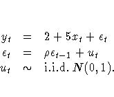
The data are generated by the following AR(1) model:
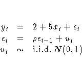
where ![]() and ut are disturbances terms. Based on this model, this example compares the finite sample efficiency of OLS and the Yule-Walker method by drawing 1000 samples with 20 observations each.
and ut are disturbances terms. Based on this model, this example compares the finite sample efficiency of OLS and the Yule-Walker method by drawing 1000 samples with 20 observations each.
Analysis
In order to compare the finite sample efficiency of OLS and the Yule-Walker method by simulation, this example generates 1000 samples of 20 observations each for the following model:
This generation of samples is accomplished by using the DATA step to turn the model into simulated data. For this example, the value of ![]() is set equal to 0.9. You can choose to repeat the experiment several times with other values of
is set equal to 0.9. You can choose to repeat the experiment several times with other values of ![]() to investigate the relative efficiency of the estimators in different error persistence environments.
to investigate the relative efficiency of the estimators in different error persistence environments.
   data sample;
      do samp = 1 to 1000;

         rho = 0.9;

            /* first error term */
         eps = rho * rannor( 47392 ) + rannor( 82745 );

         do x = 1 to 20;
            y = 2 + 5 * x + eps;
            eps=eps;
            eps = rho * eps  + rannor( 32815 );
            output;
         end;
      end;
OLS
Each sample is then estimated by OLS using the AUTOREG procedure to specify a linear regression of Y on X and a CONSTANT. The OUTEST= option creates the SAS data set EST0 that contains the parameter estimates from each of the samples. The NOPRINT option suppresses printed output. Estimates are computed for each sample by using the BY statement to specify BY-group processing.
   proc autoreg data=sample outest=est0 noprint;
      by samp;
      model y = x ;
   run;
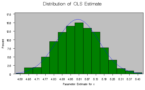
The distribution of the parameter estimates can be calculated with the UNIVARIATE procedure. The following commands rename the two variables from the SAS data set EST0 and calculate their empirical distributions.
   data estbar0;
      set est0;
      rename x=xbar0;
      rename intercep=inter0;
   run;

   proc univariate data=estbar0;
      var xbar0 ;
      histogram xbar0 / normal(color=blue) cframe=ligr
                        cfill=green;
      title 'Distribution of OLS Estimate';
   run;
Below are the summary statistics for the coefficient of X. The mean is very close to 5, the true value, and the variance is 0.022508.
 |
Yule-Walker
The Yule-Walker estimator is calculated similarly. It is chosen as the method of estimation by specifying the NLAG= option in the model statement in the AUTOREG procedure. Again, the distribution of the parameter estimates is calculated by using the UNIVARIATE procedure.
proc autoreg data=sample outest=est1 noprint;
by samp;
model y = x / nlag=1;
run;
data estbar1;
set est1;
rename x=xbar1;
rename intercep=inter1;
run;
proc univariate data=estbar1;
var xbar1 ;
histogram xbar1 / normal(color=blue) cframe=ligr
cfill=green;
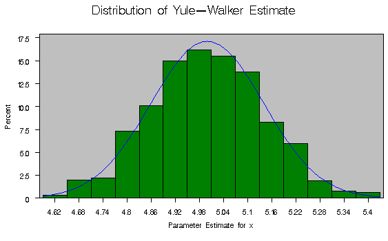
title 'Distribution of Yule-Walker Estimate';
run;
Like the OLS estimator, the mean of the Yule-Walker estimator is very close to 5. Notice, however, that the variance of the Yule-Walker estimator is 0.019559, which is less than that of the OLS estimator. Also, an examination of the quantiles reveals less dispersion in the Yule-Walker distribution as a whole.
|
||||||||||||||||||||||||||||||||||||||||||||||||||||||||||||||||||||||||||||||||||||||||||||||||||||||||||
 |
Output
The output shows that, for this experiment, the Yule-Walker estimator is slightly more efficient than the OLS estimator. The results of the standard deviations of the distribution of the parameter estimates are s2yw = 0.019559 and s2ols = 0.022508 (where s2 denotes the variance). The fact that s2yw < s2ols implies greater efficiency for the Yule-Walker method.
An F-test can be computed to see if the variances are significantly different from each other. The F statistic is the ratio of the variances for the two estimators adjusted for degrees of freedom, which is 999 for both the numerator and the denominator. The variance of the OLS estimator, s2ols, is 0.022508, while the variance of the Yule-Walker estimator, s2yw, is 0.019559. Thus, the appropriate F statistic is given by
- s2ols / s2yw = 0.022508 / 0.019559 = 1.1507746.
The p-value of this statistic for a one-sided test can be computed with the following DATA step
   data _null_;
      p = 1-probf( 1.1507746 , 999, 999 );
      put p=;
   run;
which returns a value of
- 1 - Pr F(1.1507746, 999, 999) = 0.013.
Thus, you would reject the null hypothesis that the efficiency of the two estimators is the same for most conventional levels of significance.
References
Greene, W.H. (1993), Econometric Analysis, Second Edition, New York: Macmillan Publishing Company.
Harvey, A.C. and McAvinchey, I.D. (1979), ``On the Relative Efficiency of Various Estimators of Regression Models with Moving Average Disturbances," Proceedings of the Econometric Society European Meetings, ed. E. Charatsis, Athens, 1979.
Johnston, J. (1972), Econometric Methods, Second Edition, New York: McGraw-Hill.
SAS Institute Inc. (1993), SAS/ETS User's Guide, Version 6, Second Edition, Cary, NC: SAS Institute Inc.
These sample files and code examples are provided by SAS Institute Inc. "as is" without warranty of any kind, either express or implied, including but not limited to the implied warranties of merchantability and fitness for a particular purpose. Recipients acknowledge and agree that SAS Institute shall not be liable for any damages whatsoever arising out of their use of this material. In addition, SAS Institute will provide no support for the materials contained herein.
/* Efficiency Test for Estimators by Simulation */

/*----------------------------*
   Create Monte Carlo data
 *----------------------------*/

data sample;

   rho = 0.9;

do samp = 1 to 1000;

   /* first error term */
   eps = rho * rannor( 47392 ) + rannor( 82745 );

   do x = 1 to 20;
       y = 2 + 5 * x + eps;
       eps=eps;
       eps = rho * eps  + rannor( 32815 );
       output;
   end;
end;

/*----------------------------*
      OLS estimation
 *----------------------------*/

proc autoreg data=sample outest=est0 noprint;
by samp;
model y = x ;
run;

data estbar0;
 set est0;
 rename x=xbar0;
 rename intercep=inter0;
 run;

proc univariate data=estbar0;
   var xbar0 ;
   histogram xbar0 / normal(color=blue) cframe=ligr
                     cfill=green;
   title 'Distribution of OLS Estimate';
run;

/*----------------------------*
   Yule-Walker estimation
 *----------------------------*/

proc autoreg data=sample outest=est1 noprint;
by samp;
model y = x / nlag=1;
run;

data estbar1;
 set est1;
 rename x=xbar1;
 rename intercep=inter1;
 run;

proc univariate data=estbar1;
   var xbar1 ;
   histogram xbar1 / normal(color=blue) cframe=ligr
                     cfill=green;
   title 'Distribution of Yule-Walker Estimate';
run;
These sample files and code examples are provided by SAS Institute Inc. "as is" without warranty of any kind, either express or implied, including but not limited to the implied warranties of merchantability and fitness for a particular purpose. Recipients acknowledge and agree that SAS Institute shall not be liable for any damages whatsoever arising out of their use of this material. In addition, SAS Institute will provide no support for the materials contained herein.
| Type: | Sample |
| Date Modified: | 2017-07-18 16:28:32 |
| Date Created: | 2017-07-18 13:40:31 |
Operating System and Release Information
| Product Family | Product | Host | SAS Release | |
| Starting | Ending | |||
| SAS System | SAS/ETS | z/OS | ||
| z/OS 64-bit | ||||
| OpenVMS VAX | ||||
| Microsoft® Windows® for 64-Bit Itanium-based Systems | ||||
| Microsoft Windows Server 2003 Datacenter 64-bit Edition | ||||
| Microsoft Windows Server 2003 Enterprise 64-bit Edition | ||||
| Microsoft Windows XP 64-bit Edition | ||||
| Microsoft® Windows® for x64 | ||||
| OS/2 | ||||
| Microsoft Windows 8 Enterprise 32-bit | ||||
| Microsoft Windows 8 Enterprise x64 | ||||
| Microsoft Windows 8 Pro 32-bit | ||||
| Microsoft Windows 8 Pro x64 | ||||
| Microsoft Windows 8.1 Enterprise 32-bit | ||||
| Microsoft Windows 8.1 Enterprise x64 | ||||
| Microsoft Windows 8.1 Pro 32-bit | ||||
| Microsoft Windows 8.1 Pro x64 | ||||
| Microsoft Windows 10 | ||||
| Microsoft Windows 95/98 | ||||
| Microsoft Windows 2000 Advanced Server | ||||
| Microsoft Windows 2000 Datacenter Server | ||||
| Microsoft Windows 2000 Server | ||||
| Microsoft Windows 2000 Professional | ||||
| Microsoft Windows NT Workstation | ||||
| Microsoft Windows Server 2003 Datacenter Edition | ||||
| Microsoft Windows Server 2003 Enterprise Edition | ||||
| Microsoft Windows Server 2003 Standard Edition | ||||
| Microsoft Windows Server 2003 for x64 | ||||
| Microsoft Windows Server 2008 | ||||
| Microsoft Windows Server 2008 R2 | ||||
| Microsoft Windows Server 2008 for x64 | ||||
| Microsoft Windows Server 2012 Datacenter | ||||
| Microsoft Windows Server 2012 R2 Datacenter | ||||
| Microsoft Windows Server 2012 R2 Std | ||||
| Microsoft Windows Server 2012 Std | ||||
| Microsoft Windows XP Professional | ||||
| Windows 7 Enterprise 32 bit | ||||
| Windows 7 Enterprise x64 | ||||
| Windows 7 Home Premium 32 bit | ||||
| Windows 7 Home Premium x64 | ||||
| Windows 7 Professional 32 bit | ||||
| Windows 7 Professional x64 | ||||
| Windows 7 Ultimate 32 bit | ||||
| Windows 7 Ultimate x64 | ||||
| Windows Millennium Edition (Me) | ||||
| Windows Vista | ||||
| Windows Vista for x64 | ||||
| 64-bit Enabled AIX | ||||
| 64-bit Enabled HP-UX | ||||
| 64-bit Enabled Solaris | ||||
| ABI+ for Intel Architecture | ||||
| AIX | ||||
| HP-UX | ||||
| HP-UX IPF | ||||
| IRIX | ||||
| Linux | ||||
| Linux for x64 | ||||
| Linux on Itanium | ||||
| OpenVMS Alpha | ||||
| OpenVMS on HP Integrity | ||||
| Solaris | ||||
| Solaris for x64 | ||||
| Tru64 UNIX | ||||