In a test of equivalence, the means for a new and a reference treatment are compared to try to show that the treatments are the same. Equivalence tests are often used in bioequivalence studies in which two drugs are compared with the intent to show that the new drug is the same as a standard drug.

Under the null hypothesis of an equivalence test, the treatment means differ by more than some practically unimportant amount called the margin. Under the alternative hypothesis, the means differ by less than this amount and are therefore considered equivalent for practical purposes. Since the power of a test is the probability of rejecting the null hypothesis when the alternative is true, the power in an equivalence test is the probability of rejecting nonequivalence when the treatments are in fact equivalent. That is, it is the probability of observing a difference (or ratio) of treatment means within the margin when the true values are within the margin. Equivalence tests are further introduced along with the related inferiority and superiority tests in SAS Note 48616.

Design and Analysis Tools for Equivalence Tests

Power analysis and sample size determination for equivalence tests can be done in PROC POWER for the following situations. Analysis of data from an equivalence study can be conducted using PROC FREQ or PROC TTEST:

Type of Test	PROC POWER Statement	Analysis Procedure	Required Statement
One-sample test of mean	ONESAMPLEMEANS	TTEST
Two-sample comparison of means	TWOSAMPLEMEANS	TTEST	CLASS
Paired-sample comparison of means	PAIREDMEANS	TTEST	PAIRED
One-sample test of proportion	ONESAMPLEFREQ	FREQ	TABLE BINOMIAL(EQUIV P= MARGIN=)
Two-sample comparison of proportions	Not available	FREQ	TABLE RISKDIFF(EQUIV MARGIN=)
Paired-sample comparison of proportions		Not available

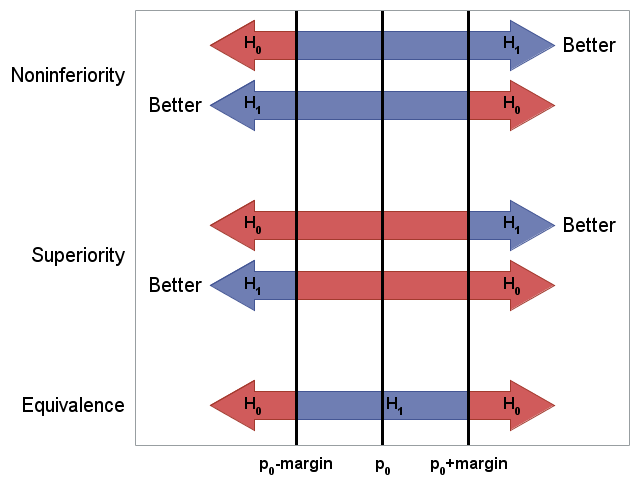
The following graph repeats the visualization of equivalence, noninferiority, and superiority tests as seen in SAS Note 48616. It shows how these tests differ with respect to the direction of desirable outcome and contents of the null and alternative hypotheses. (See the SAS code that produces this graph.)

The following examples illustrate designing equivalence studies and conducting equivalence tests. Additional examples of power and sample size computations for equivalence tests using the ONESAMPLEMEANS, TWOSAMPLEMEANS, PAIREDMEANS, and ONESAMPLEFREQ statements are available in the descriptions of these statements in the PROC POWER documentation.

One-Sample Equivalence Test: The ONESAMPLEMEANS Statement

Suppose a cereal company wants to test whether a new packaging machine produces boxes with weight equivalent to a target value of 14 ounces per box. Weight is assumed to be normally distributed and the researchers decide that a meaningful difference from the target must exceed 0.2 oz. in either direction. The standard deviation of the weight is about 0.5 oz. What is the sample size needed in an 0.05 level equivalence test with 90% power to conclude the weight is within the margin?

The hypotheses for a one-sample equivalence test are:

H₀: μ < θ_L or μ > θ_U
H₁: θ_L ≤ μ ≤ θ_U

where μ is the mean weight from the new machine. With target value μ₀ and margin m, θ_L=μ₀-m and θ_U=μ₀+m are the lower and upper bounds specified in the LOWER= and UPPER= options in the ONESAMPLEMEANS statement in PROC POWER. Following the two one-sided tests (TOST) procedure of Schuirmann (1987), the equivalence test is conducted by performing two separate tests, L and U:

H_0L: μ < θ_L
H_1L: μ ≥ θ_L

and

H_0U: μ > θ_U
H_1U: μ ≤ θ_U

The overall p-value of the equivalence test is the larger of the two p-values of tests L and U. Rejection of H₀ in favor of H₁ at significance level α occurs if and only if the 100(1-2α)% confidence interval for μ is contained completely within (θ_L, θ_U).

For this example with μ₀=14 and m=0.2, the hypotheses are as follows:

H₀: μ < 13.8 or μ > 14.2
H₁: 13.8 ≤ μ ≤ 14.2

The following statements compute the sample size for this equivalence test:

      proc power;
         onesamplemeans test=equiv
            lower  = 13.8
            upper  = 14.2
            mean   = 14
            stddev = 0.5
            ntotal = .
            power  = 0.9
            alpha  = 0.05;
         run;

The results show that a sample size of 70 is required to have 90% power for this equivalence test:

The POWER Procedure Equivalence Test for Normal Mean Fixed Scenario Elements Distribution Normal Method Exact Lower Equivalence Bound 13.8 Upper Equivalence Bound 14.2 Alpha 0.05 Mean 14 Standard Deviation 0.5 Nominal Power 0.9 Computed N Total Actual Power N Total 0.905 70

Suppose weight measurements are obtained from 70 randomly selected cereal boxes. These statements create a data set of the observed box weights:

      data BoxWts;
         input weight @@;
         datalines;
      14.15   13.68   13.58   14.26   14.29
      14.32   13.56   14.03   12.68   13.58
      14.13   14.37   14.11   13.94   14.11
      14.27   13.92   14.50   14.05   13.77
      14.60   14.18   14.07   14.15   13.82
      13.76   14.28   13.67   14.58   14.83
      13.71   13.31   13.46   14.12   14.14
      13.05   14.08   13.98   14.04   14.33
      13.42   14.00   13.70   14.09   14.12
      13.48   13.70   14.11   14.14   13.17
      13.82   13.55   13.54   13.11   13.92
      13.56   14.08   13.17   14.52   14.23
      14.22   13.82   13.64   14.32   14.31
      13.55   13.58   13.25   14.34   14.02
	  

The following statements use PROC TTEST to perform the equivalence test. The TOST option requests the two one-sided equivalence test. The equivalence bounds are specified in parentheses:

      proc ttest data=BoxWts tost(13.8, 14.2);
         var weight;
         run;

The average weight of the sampled boxes is 13.91 oz. The equivalence test finds significant evidence that the true mean weight is equivalent to the target (p=0.0124). This is visually apparent since the 90% confidence interval (13.83, 14.00) on the mean weight is completely contained within the equivalence bounds:

TOST Level 0.05 Equivalence Analysis Mean Lower Bound   90% CL Mean   Upper Bound Assessment 13.9134 13.8 < 13.8311 13.9958 < 14.2 Equivalent Test Null DF t Value P-Value Upper 13.8 69 2.30 0.0124 Lower 14.2 69 -5.80 <.0001 Overall       0.0124

Paired-Sample Equivalence Test: The PAIREDMEANS Statement

In a study hoping to show that exposure to a substance has no effect on subjects, subject responses are recorded before and after exposure. The response values are assumed to have a lognormal distribution. A 0.05 level equivalence test with 90% power is proposed to test that the ratio of the mean responses is within equivalence bounds [0.8, 1.25]. The correlation between the measurements within subjects is assumed to be 0.6 based on previous similar studies. It is desired to explore the sample sizes needed for a range of CV (Coefficient of Variation = standard deviation / mean) values common to both groups. Based on prior knowledge of this substance, a range of CV values between 0.2 and 0.3 is assumed, and a range of possible mean ratios from 0.85 to 1.15 is of interest.

The mean ratio refers to the ratio of the geometric means from the two groups. For definitions of arithmetic and geometric means, see "Computational Methods: Arithmetic and Geometric Means" in the Details section of the TTEST procedure documentation. Along with the correlation, the CV specifies the variability in lognormal data. The CV is assumed to be common to both groups, and the standard deviation and mean in the CV formula are the arithmetic mean and standard deviation of the original data. CV relates to the variance of the log-transformed data, v, as CV = sqrt(exp(v)-1). See "Computational Methods: Coefficient of Variation" in the Details section of the TTEST documentation for more information.

The following statements compute and plot the sample sizes for several CV-mean ratio scenarios using the PAIREDMEANS statement. The TEST=EQUIV_RATIO option requests power analysis for an equivalence test based on the ratio of means. Note that for an equivalence test the specified ALPHA= value provides the sample size for a (1-2α)100% confidence interval on the mean ratio. The PLOT statement plots the number of pairs needed for each of the scenarios:

      proc power; 
         pairedmeans test=equiv_ratio 
            lower     = 0.8 
            upper     = 1.25 
            meanratio = 0.85 to 1.15 by 0.05 
            cv        = 0.2 0.23 0.25 0.3
            corr      = 0.6 
            npairs    = . 
            alpha     = 0.05 
            power     = 0.90; 
         plot x=effect step=0.05 
              vary(color by cv) yopts=(ref=10 to 170 by 10); 
         run;

Results of the power analysis shows that the larger the CV or the farther the mean ratio is from 1, the larger sample size required for the equivalence test:

The POWER Procedure Equivalence Test for Paired Mean Ratio

Suppose researchers decide that the most likely CV and mean ratio values will call for a sample size of 20. They proceed to conduct the study with 20 patients and the resulting measurements from each subject before and after exposure are recorded in the following data set:

      data Responses;
         input Subject Before After @@;
         datalines;
       1  21.84  25.05    11  18.41  23.87
       2  22.42  24.22    12  26.21  26.02
       3  20.38  23.85    13  19.11  21.88
       4  20.30  16.61    14  16.51  22.26
       5  19.08  22.04    15  26.15  20.21
       6  22.35  29.32    16  16.78  20.13
       7  19.63  17.55    17  18.67  19.44
       8  21.18  16.94    18  22.14  22.61
       9  24.75  22.70    19  22.37  22.45
      10  14.45  11.27    20  20.33  22.84
      

The equivalence test for paired samples is performed using the PAIRED statement in PROC TTEST:

      proc ttest data=Responses dist=lognormal tost(0.8, 1.25);
         paired before*after;
         run;

The nonequivalence null hypothesis is rejected (p<0.0001) indicating significant evidence for equivalent means before and after exposure and implying no effect due to exposure to the substance:

TOST Level 0.05 Equivalence Analysis Geometric Mean Lower Bound   90% CL Mean   Upper Bound Assessment 0.9652 0.8 < 0.9021 1.0327 < 1.25 Equivalent Test Null DF t Value P-Value Upper 0.8 19 4.80 <.0001 Lower 1.25 19 -6.61 <.0001 Overall       <.0001

 

One-Sample Equivalence Test: The ONESAMPLEFREQ Statement

For a popular toothpaste, noticeable whitening of the teeth has been shown in 30% of customers after one month of use of this product. Another company wants to show that their less expensive toothpaste produces an equivalent whitening effect. The company decides that equivalence requires that they differ by no more than 10%. In early testing of the new toothpaste, 35% of its customers reported noticeable whitening after one month of use. Assuming the new toothpaste produces 35% whitening, what is the sample size needed in a new study for a 0.05 level equivalence test with 90% power to conclude the whitening effect is within the margin?

The hypotheses for a one-sample equivalence test are as follows:

H₀: p ≤ θ_L or p ≥ θ_U
H₁: θ_L< p <θ_U

where p is the proportion with noticeable whitening. With target value p₀ and margin m, θ_L=p₀-m and θ_U=p₀+m are the lower and upper bounds. Rejection of H₀ in favor of H₁ at significance level α occurs if and only if the 100(1-2α)% confidence interval for p is contained completely within (θ_L, θ_U).

For this example with p₀=0.3 and m=0.1, the hypotheses are as follows:

H₀: p < 0.2 or p > 0.4
H₁: 0.2 ≤ p ≤ 0.4

Three equivalence tests are available in PROC POWER: EQUIV_EXACT, EQUIV_Z, EQUIV_ADJZ. See the table of available tests and appropriate syntax in the table below. Detailed information about these tests is provided in the Details section of the PROC POWER documentation.

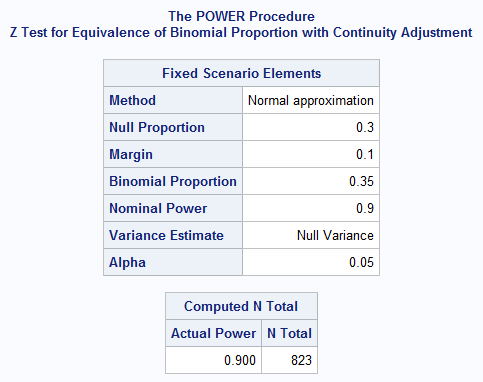
The following statements compute the sample size for an equivalence test based on the normal-approximate z statistic with continuity adjustment using the two one-sided tests (TOST) method and with variance based on the probability in the null hypothesis:

   proc power;
      onesamplefreq test=equiv_adjz method=normal
         proportion = 0.35
         nullproportion = 0.3
         margin = 0.1
         ntotal = .
         power = .9;
      run;

The results show that a sample size of 823 is required to have 90% power for this 0.05 level equivalence test:

Based on the above power analysis, suppose a study is conducted with 823 customers and the outcome of noticeable whitening after one month of use is recorded. The summarized data set is created in the following statements:

   data study;
      input outcome count;
      datalines;
   1 296
   0 527
   ;

The following statements use PROC FREQ to perform the equivalence test described above. The EQUIV option requests a test of equivalence for the binomial proportion. The P= option specifies the proportion in the null hypothesis. The MARGIN= option specifies the equivalence margin.

Since TEST=EQUIV_ADJZ was used in PROC POWER specifying a continuity corrected test, the CORRECT option is specified in PROC FREQ. If you specify TEST=EQUIV_Z in PROC POWER, the CORRECT option is not needed in PROC FREQ. Note that the variance used in PROC POWER by default is based on the null proportion. To match this, it is necessary to specify VAR=NULL in PROC FREQ. Alternatively, if VAREST=SAMPLE was specified in PROC POWER, the default VAR=SAMPLE could be used in PROC FREQ:

   proc freq data=study;
      tables outcome / binomial(level='1' equiv p=.30 margin=.1
                       correct var=null);
      weight Count;
      run;

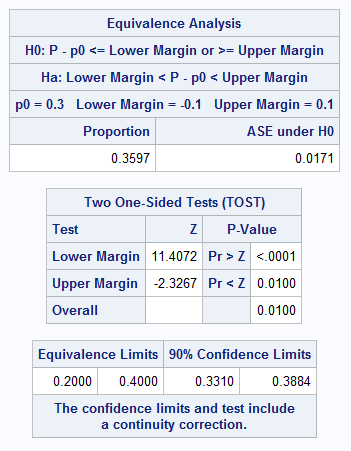
Since the Overall p-value in the "Two One-Sided Tests (TOST)" table is significant at the predetermined 0.05 level, the null hypothesis is rejected in favor of the equivalence hypothesis (p=0.0100):

 

Available equivalence tests and their syntax for power and analysis

 

The following table shows the additional options to specify in the POWER and FREQ procedures for the same equivalence test. In the ONESAMPLEFREQ statement in PROC POWER, all equivalence tests should include the PROPORTION= option and either the EQUIVBOUNDS= option, or both the MARGIN= and NULLPROPORTION= options, or both the LOWER= and UPPER= options. In the TABLES statement in PROC FREQ, all equivalence tests should include EQUIV, P=, and MARGIN= in the BINOMIAL option. If needed to select the event level, also include LEVEL=. For the exact test, the EXACT BINOMIAL; statement must be included.

Note that when the exact test is requested in PROC POWER, it is not possible to solve directly for the sample size. See the example below which shows a way to find a suitable sample size. Also note that exact tests based on the z statistic are not available in PROC FREQ.

 

Equivalence Tests For One-Sample Proportion

 

Test	Method Exact or Normal	Continuity Correction Yes or No	Variance Null or Sample	Additional PROC POWER ONESAMPLEFREQ Syntax	Additional PROC FREQ BINOMIAL Syntax
Z	Normal	No	Null	TEST=EQUIV_Z METHOD=NORMAL VAREST=NULL	VAR=NULL
Z	Normal	No	Sample	TEST=EQUIV_Z METHOD=NORMAL VAREST=SAMPLE	VAR=SAMPLE
Adjusted Z	Normal	Yes	Null	TEST=EQUIV_ADJZ METHOD=NORMAL VAREST=NULL	CORRECT VAR=NULL
Adjusted Z	Normal	Yes	Sample	TEST=EQUIV_ADJZ METHOD=NORMAL VAREST=SAMPLE	CORRECT VAR=SAMPLE
Exact	Exact	n/a	n/a	TEST=EQUIV_EXACT	See NOTE below
Z	Exact	No	Null	TEST=EQUIV_Z METHOD=EXACT VAREST=NULL	n/a
Z	Exact	No	Sample	TEST=EQUIV_Z METHOD=EXACT VAREST=SAMPLE	n/a
Adjusted Z	Exact	Yes	Null	TEST=EQUIV_ADJZ METHOD=EXACT VAREST=NULL	n/a
Adjusted Z	Exact	Yes	Sample	TEST=EQUIV_ADJZ METHOD=EXACT VAREST=SAMPLE	n/a

NOTE: To perform the EXACT equivalence test in PROC FREQ, the EXACT BINOMIAL; statement is required as shown in the following example.

 

Finding sample size for the exact equivalence test

 

As noted above, you cannot solve for NTOTAL using the exact method specified by the TEST=EQUIV_EXACT option (which implies METHOD=EXACT). If you prefer to use the exact method, you can determine sample size by entering a range of sample sizes and then use PROC POWER to solve for power at each size. Select the sample size that results in the power closest to the desired power.

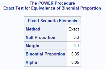
The following statements use the exact method to search for a suitable sample size for the two-sided equivalence test based on the two one-sided tests (TOST) method:

   proc power;
      onesamplefreq test=equiv_exact
         proportion = 0.35
         nullproportion = 0.3
         margin = 0.1
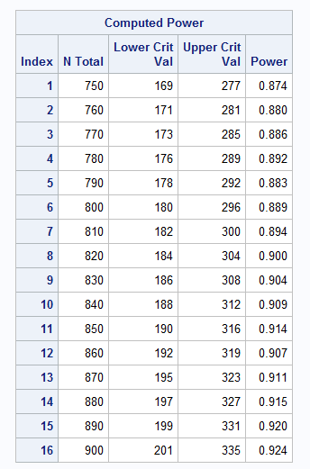
         ntotal = 750 to 900 by 10
         power = .;
      run;

The output shows that a sample size of 820 yields an exact equivalence test with power equal to 0.9. Note that this is about the same as the sample size found in the example above using the normal-approximate, adjusted z test:

If 820 observations are collected, the following statements can be used to conduct the exact equivalence test:

   proc freq data=test;
      tables outcome / binomial(level='1' equiv p=.30 margin=.1);
      exact binomial;
      weight Count;
      run;

Operating System and Release Information

Product Family	Product	System	SAS Release
			Reported	Fixed*
SAS System	SAS/STAT	Microsoft® Windows® for 64-Bit Itanium-based Systems
		Z64
		z/OS
		OpenVMS VAX
		Microsoft Windows Server 2003 Datacenter 64-bit Edition
		Microsoft Windows Server 2003 Enterprise 64-bit Edition
		Microsoft Windows XP 64-bit Edition
		Microsoft® Windows® for x64
		OS/2
		Microsoft Windows 8 Enterprise 32-bit
		Microsoft Windows 8 Enterprise x64
		Microsoft Windows 8 Pro 32-bit
		Microsoft Windows 8 Pro x64
		Microsoft Windows 95/98
		Microsoft Windows 2000 Advanced Server
		Microsoft Windows 2000 Datacenter Server
		Microsoft Windows 2000 Server
		Microsoft Windows 2000 Professional
		Microsoft Windows NT Workstation
		Microsoft Windows Server 2003 Datacenter Edition
		Microsoft Windows Server 2003 Enterprise Edition
		Microsoft Windows Server 2003 Standard Edition
		Microsoft Windows Server 2003 for x64
		Microsoft Windows Server 2008
		Microsoft Windows Server 2008 R2
		Microsoft Windows Server 2008 for x64
		Microsoft Windows Server 2012 Datacenter
		Microsoft Windows Server 2012 Std
		Microsoft Windows XP Professional
		Windows 7 Enterprise 32 bit
		Windows 7 Enterprise x64
		Windows 7 Home Premium 32 bit
		Windows 7 Home Premium x64
		Windows 7 Professional 32 bit
		Windows 7 Professional x64
		Windows 7 Ultimate 32 bit
		Windows 7 Ultimate x64
		Windows Millennium Edition (Me)
		Windows Vista
		Windows Vista for x64
		64-bit Enabled AIX
		64-bit Enabled HP-UX
		64-bit Enabled Solaris
		ABI+ for Intel Architecture
		AIX
		HP-UX
		HP-UX IPF
		IRIX
		Linux
		Linux for x64
		Linux on Itanium
		OpenVMS Alpha
		OpenVMS on HP Integrity
		Solaris
		Solaris for x64
		Tru64 UNIX

* For software releases that are not yet generally available, the Fixed Release is the software release in which the problem is planned to be fixed.

---

proc power;
         onesamplemeans test=equiv
            lower  = 13.8
            upper  = 14.2
            mean   = 14
            stddev = 0.5
            ntotal = .
            power  = 0.9
            alpha  = 0.05;
         run;

 data BoxWts;
         input weight @@;
         datalines;
      14.15   13.68   13.58   14.26   14.29
      14.32   13.56   14.03   12.68   13.58
      14.13   14.37   14.11   13.94   14.11
      14.27   13.92   14.50   14.05   13.77
      14.60   14.18   14.07   14.15   13.82
      13.76   14.28   13.67   14.58   14.83
      13.71   13.31   13.46   14.12   14.14
      13.05   14.08   13.98   14.04   14.33
      13.42   14.00   13.70   14.09   14.12
      13.48   13.70   14.11   14.14   13.17
      13.82   13.55   13.54   13.11   13.92
      13.56   14.08   13.17   14.52   14.23
      14.22   13.82   13.64   14.32   14.31
      13.55   13.58   13.25   14.34   14.02
	  ;

      proc ttest data=BoxWts tost(13.8, 14.2);
         var weight;
         run;

proc power; 
         pairedmeans test=equiv_ratio 
            lower     = 0.8 
            upper     = 1.25 
            meanratio = 0.85 to 1.15 by 0.05 
            cv        = 0.2 0.23 0.25 0.3
            corr      = 0.6 
            npairs    = . 
            alpha     = 0.05 
            power     = 0.90; 
         plot x=effect step=0.05 
              vary(color by cv) yopts=(ref=10 to 170 by 10); 
         run;


		 data Responses;
         input Subject Before After @@;
         datalines;
       1  21.84  25.05    11  18.41  23.87
       2  22.42  24.22    12  26.21  26.02
       3  20.38  23.85    13  19.11  21.88
       4  20.30  16.61    14  16.51  22.26
       5  19.08  22.04    15  26.15  20.21
       6  22.35  29.32    16  16.78  20.13
       7  19.63  17.55    17  18.67  19.44
       8  21.18  16.94    18  22.14  22.61
       9  24.75  22.70    19  22.37  22.45
      10  14.45  11.27    20  20.33  22.84
      ;

      proc ttest data=Responses dist=lognormal tost(0.8, 1.25);
         paired before*after;
         run;

proc power;
  onesamplefreq test=equiv_adjz method=normal
  proportion = 0.35
  nullproportion = 0.3
  margin = 0.1
  ntotal = .
  power = .9;
run;


proc power;
   onesamplefreq test=equiv_exact
   proportion = 0.35
   nullproportion = 0.3
   margin = 0.1
   ntotal = 700 to 900 by 10
   power = .;
run;


data Color; 
  input Hair $ Count @@;
  label Hair='Hair Color';
datalines;
fair   23    red      7    medium 24
dark   11    fair    19    red     7
medium 18    dark    14    fair   34
red     5    medium  41    dark   40
black   3    fair    46    red    21
medium 44    dark    40    black   6
fair   50    red     31    medium 37
dark   23    fair    56    red    42
medium 53    dark    54    black  13
;

proc freq data=Color ;
   tables Hair / binomial(level='Fair' equiv p=.30 margin=.1);
   weight Count;
run;


data BB;
 do group=1 to 2;
  input p0 p1;
    y=0; py=p0/(p0+p1); output;
    y=1; py=p1/(p0+p1); output;
  end;
  datalines;
.2 .05
.225 .025
;

proc freq data=bb;
 weight py;
 table group*y;
run;

proc freq data=bb;
 weight py;
 table group*y/riskdiff (equiv margin=0.25);
 ods output PdiffEquivTest=equv;
run;

proc sort; by descending pvalue; run;

data _null_;
  set equv;
  call symput('z',cats(z/2));
  stop;
run;

proc power;
custom
  dist=normal
  primnc=&z
  ntotal=.
  power=0.8;
run;

Type:	Usage Note
Priority:
Topic:	Analytics ==> Power and Sample Size SAS Reference ==> Procedures ==> POWER SAS Reference ==> Procedures ==> TTEST

Date Modified:	2025-11-13 16:01:15
Date Created:	2013-08-08 15:15:22