45581 - Bayesian Binomial Model with Power Prior Using the MCMC Procedure

Sample 45581: Bayesian Binomial Model with Power Prior Using the MCMC Procedure

PDF of Example | SAS/STAT Focus Area Examples

Analysis

Suppose that, in addition to data from a current study, you have similar data from a historical data set or pilot study. A power prior enables you to capture the information collected in the pilot study and incorporate it into analysis and inference in the current study. The historical data gets integrated via an informative prior and provides a convenient way of updating past knowledge.

A power prior can be expressed as a product of the weighted likelihood of $\text{[math]}$ conditional on the historical data and a prior distribution on the parameters before any data is observed. More formally, the power prior distribution of $\text{[math]}$ is written as

$\text{[math]}$

where $\text{[math]}$ are the historical data (from the pilot study), $\text{[math]}$ is the likelihood of $\text{[math]}$ conditional on historical data, $\text{[math]}$ is a discounting or scale parameter with $\text{[math]}$ that controls the amount of weight you want to put on the historical data, and $\text{[math]}$ is a prior for $\text{[math]}$ before the historical data $\text{[math]}$ are observed.

The posterior distribution of $\text{[math]}$ is

$\text{[math]}$	$\text{[math]}$	$\text{[math]}$
$\text{[math]}$	$\text{[math]}$	$\text{[math]}$
$\text{[math]}$	$\text{[math]}$	$\text{[math]}$	( 1 )

where $\text{[math]}$ represents the data from the current study, $\text{[math]}$ for $\text{[math]}$ , $\text{[math]}$ for $\text{[math]}$ represents the historical data, and $\text{[math]}$ represents the density function for a single observation in either the historical or the current data set.

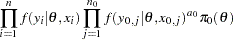
You can combine the two data sets to form a new data set $\text{[math]}$ and rewrite the posterior distribution in Equation 1 as the following:

	$\text{[math]}$	$\text{[math]}$	$\text{[math]}$		( 2 )
	$\text{[math]}$	$\text{[math]}$	$\text{[math]}$

The posterior distribution Equation 2 is used to model the hypothetical clinical trial setting described in this example. The following SAS statements create the PTRIALS data set that represents binomial data collected in a pilot study of a clinical trial.

      data ptrials;
         input y n;
         datalines;
      5 163
      ;

In the INPUT statement, $\text{[math]}$ represents the number of successes out of $\text{[math]}$ independent Bernoulli trials. Similarly, for the current study, suppose you have the following hypothetical clinical trials data set BTRIALS .

      data btrials;
         input y n @@;
         datalines;
      2  86
      2  69
      1  71
      1 113
      1 103
      ;

In order to fit a model with a power prior, first combine both the current and pilot study data sets. The indicator GROUP variable takes on the values ' CURRENT ' and ' PILOT ' for the current and pilot study data set, respectively. The following SAS statements demonstrate how to create a new combined data set ALLDATA .

      data alldata;
         set btrials(in=i) ptrials;
         if i then group='current';
         else group = 'pilot';
      run;

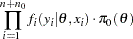
Suppose you want to fit a Bayesian binomial model with a power prior for a hypothetical clinical trial setting with density

$\text{[math]}$

( 3 )

where $\text{[math]}$ is the success probability for $\text{[math]}$ observations.

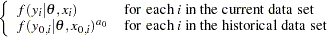
The likelihood function for each of the observations is

$\text{[math]}$

( 4 )

where $\text{[math]}$ denotes a conditional probability mass function. The binomial density is evaluated at the specified value of $\text{[math]}$ and corresponding success probability $\text{[math]}$ . Then, a power prior is used to assign each observation in the combined data set a binomial or weighted binomial likelihood function depending whether the observation was from the current or pilot study, respectively.

Suppose the following power prior is placed on the success probability parameters, where $\text{[math]}$ represents the binomial likelihood:

$\text{[math]}$	$\text{[math]}$	$\text{[math]}$
$\text{[math]}$	$\text{[math]}$	$\text{[math]}$
$\text{[math]}$	$\text{[math]}$	$\text{[math]}$	( 5 )

The variables $\text{[math]}$ and $\text{[math]}$ represent the historical successes and sample size, respectively, and $\text{[math]}$ indicates a prior distribution. Suppose for this example that the discounting factor is set to $\text{[math]}$ . The diffuse $\text{[math]}$ prior expresses your lack of knowledge about the success probability.

According to Bayes’ theorem, the likelihood function and prior distribution determine the posterior distribution of $\text{[math]}$ as given in Equation 2 . PROC MCMC obtains samples from the desired posterior distribution, which is determined by the specified prior and likelihood. It does not require the exact form of the posterior distribution.

The following SAS statements use the likelihood and power prior distribution to fit the Bayesian binomial model with the historical data. The PROC MCMC statement invokes the procedure and specifies the input data set. The SEED= option specifies a seed for the random number generator, which guarantees the reproducibility of the random stream. The NMC= option specifies the number of posterior simulation iterations.

   ods graphics on;
   proc mcmc data=alldata seed=1181 nmc=10000;
      parms p 0.2;
      begincnst;
         a0 = 0.5;
      endcnst;
      prior p ~ uniform(0,1);
      llike = logpdf('binomial',y,p,n);
      if (group='pilot') then llike = a0*llike;
      model general(llike);
   run;     
   ods graphics off;

The PARMS statement designates $\text{[math]}$ as a parameter in the model and assigns an initial value of 0.2 to it. The programming statements enclosed by the BEGINCNST and ENDCNST statements are executed once per procedure call and designate the discount factor for the power prior.

The PRIOR statement specifies a prior $\text{[math]}$ as given in Equation 5 . The LLIKE= assignment statement assigns the log-likelihood function for $\text{[math]}$ as given in Equation 3 ; the LOGPDF function calculates the logarithm of the binomial function. The IF/THEN statement uses the GROUP indicator variable to weight the binomial likelihood when the observation is from the pilot study.

The MODEL statement uses the GENERAL function, which indicates that you are using a SAS statement to construct a nonstandard density or distribution. The argument is an expression that takes the value of the logarithm function of the prior or likelihood distribution. In this case, the nonstandard density is the binomial or weighted binomial likelihood, and the argument is the logarithm of the density.

Figure 1 displays convergence diagnostic plots for $\text{[math]}$ to assess whether the Markov chains have converged. Inferences should not be made if the Markov chain has not converged.

Figure 1 Bayesian Binomial Model Diagnostic Plots for $\text{[math]}$

Bayesian Binomial Model Diagnostic Plots for p

The trace plot shows that the mean of the Markov chain is constant over the graph and is stabilized. The chain is able to traverse the support of the target distribution, and the mixing is good. The trace plot shows that the Markov chain appears to have reached a stationary distribution.

The autocorrelation plot indicates low autocorrelation and efficient sampling. The kernel density plot shows a smooth, unimodal posterior marginal distribution for the parameter.

PROC MCMC produces formal diagnostic tests by default, but they are omitted here because informal checks on the chains, autocorrelation, and posterior density plots show desired stabilization and convergence.

Figure 2 reports summary and interval statistics for the parameter’s posterior distribution.

Figure 2 Posterior Model Summary of Binomial Model

The MCMC Procedure

Posterior Summaries
Parameter	N	Mean	Standard Deviation	Percentiles
Parameter	N	Mean	Standard Deviation	25%	50%	75%
p	10000	0.0200	0.00602	0.0156	0.0194	0.0237

Posterior Intervals
Parameter	Alpha	Equal-Tail Interval		HPD Interval
p	0.050	0.0100	0.0333	0.00900	0.0316

Using the power prior, the posterior mean of the success probability is 2.00% with a 95% credible interval of $\text{[math]}$ , providing evidence of a treatment effect.

Modeling the clinical trial data set in a Bayesian binomial model with a power prior is a good way to make use of the pilot study. It enables you to use a different class of informative priors and incorporates relevant historical data and information.

References

Ibrahim, J. G. and Chen, M.-H. (2000), “Power Prior Distributions for Regression Models,” Statistical Science , 15, 46–60.

These sample files and code examples are provided by SAS Institute Inc. "as is" without warranty of any kind, either express or implied, including but not limited to the implied warranties of merchantability and fitness for a particular purpose. Recipients acknowledge and agree that SAS Institute shall not be liable for any damages whatsoever arising out of their use of this material. In addition, SAS Institute will provide no support for the materials contained herein.


   data ptrials;
      input y n;
      datalines;
   5 163
   ; 


   data btrials;
      input y n @@;
      datalines;
   2  86
   2  69
   1  71
   1 113
   1 103
   ;


   data alldata;
      set btrials(in=i) ptrials;
      if i then group='current';
      else group = 'pilot';
   run;


ods graphics on;
proc mcmc data=alldata seed=1181 nmc=10000;
   parms p 0.2;
   begincnst;
      a0 = 0.5;
   endcnst;
   prior p ~ uniform(0,1);
   llike = logpdf('binomial',y,p,n);
   if (group='pilot') then llike = a0*llike;
   model general(llike);
run;     
ods graphics off;

These sample files and code examples are provided by SAS Institute Inc. "as is" without warranty of any kind, either express or implied, including but not limited to the implied warranties of merchantability and fitness for a particular purpose. Recipients acknowledge and agree that SAS Institute shall not be liable for any damages whatsoever arising out of their use of this material. In addition, SAS Institute will provide no support for the materials contained herein.

Type:	Sample
Topic:	Analytics ==> Bayesian Analysis SAS Reference ==> Procedures ==> MCMC

Date Modified:	2016-08-02 13:31:11
Date Created:	2012-02-06 12:26:32

Product Family	Product	Host	SAS Release
Product Family	Product	Host	Starting	Ending
SAS System	SAS/STAT	z/OS
		OpenVMS VAX
		Microsoft® Windows® for 64-Bit Itanium-based Systems
		Microsoft Windows Server 2003 Datacenter 64-bit Edition
		Microsoft Windows Server 2003 Enterprise 64-bit Edition
		Microsoft Windows XP 64-bit Edition
		Microsoft® Windows® for x64
		OS/2
		Microsoft Windows 95/98
		Microsoft Windows 2000 Advanced Server
		Microsoft Windows 2000 Datacenter Server
		Microsoft Windows 2000 Server
		Microsoft Windows 2000 Professional
		Microsoft Windows NT Workstation
		Microsoft Windows Server 2003 Datacenter Edition
		Microsoft Windows Server 2003 Enterprise Edition
		Microsoft Windows Server 2003 Standard Edition
		Microsoft Windows Server 2003 for x64
		Microsoft Windows Server 2008
		Microsoft Windows Server 2008 for x64
		Microsoft Windows XP Professional
		Windows 7 Enterprise 32 bit
		Windows 7 Enterprise x64
		Windows 7 Home Premium 32 bit
		Windows 7 Home Premium x64
		Windows 7 Professional 32 bit
		Windows 7 Professional x64
		Windows 7 Ultimate 32 bit
		Windows 7 Ultimate x64
		Windows Millennium Edition (Me)
		Windows Vista
		Windows Vista for x64
		64-bit Enabled AIX
		64-bit Enabled HP-UX
		64-bit Enabled Solaris
		ABI+ for Intel Architecture
		AIX
		HP-UX
		HP-UX IPF
		IRIX
		Linux
		Linux for x64
		Linux on Itanium
		OpenVMS Alpha
		OpenVMS on HP Integrity
		Solaris
		Solaris for x64
		Tru64 UNIX

Support

Sample 45581: Bayesian Binomial Model with Power Prior Using the MCMC Procedure

Analysis

References

Operating System and Release Information