Usage Note 37110: Plotting the fitted values from a random coefficients model
 |  |  |
After fitting a random coefficients model (also called a hierarchical linear model or HLM), you may want to graph the resulting fitted regression model for each subject. Specify the OUTP= option in the MODEL statement of PROC MIXED to create a data set containing predicted values. Beginning in SAS 9.2, you can use PROC SGPLOT to plot the model. PROC GPLOT can also produce the plot.
Below is an example of fitting and plotting a random coefficients model. For more information about random coefficients models and how to obtain estimates and tests for the subject-specific regression coefficients in these models, see this note.
The following data set contains data for five randomly selected wheat varieties. Each variety was assigned to six one-acre plots of land. From each plot of land, the yield and the amount of moisture were measured.
      data wheat;
         input id variety yield moist;
         datalines;
       1       1         41       10
       2       1         69       57
       3       1         53       32
       4       1         66       52
       5       1         64       47
       6       1         64       48
       7       2         49       30
       8       2         44       21
       9       2         44       20
      10       2         46       26
      11       2         57       44
      12       2         42       19
      13       3         69       50
      14       3         62       40
      15       3         50       23
      16       3         76       58
      17       3         48       21
      18       3         55       30
      19       4         48       22
      20       4         60       40
      21       4         45       17
      22       4         47       21
      23       4         62       44
      24       4         43       13
      25       5         65       49
      26       5         63       44
      27       5         71       57
      28       5         68       51
      29       5         52       27
      30       5         68       52
      ;
The following statements fit the random coefficients model as discussed in this note.
      proc mixed data=wheat;
         class variety;
         model yield = moist / ddfm=kr solution outp=pred;
         random int moist / type=un subject=variety solution;
         run;
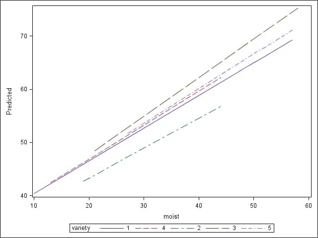
PROC SGPLOT can be used to plot the fitted values from the model. The vertical (Y) and horizontal (X) axis variables are specified in the SERIES statement. The GROUP= option causes a line to be displayed for each level of the specified variable. The data are sorted prior to plotting so that each line is drawn from minimum to maximum MOIST value, preventing any overdrawing of the lines.
      proc sort data=pred;
         by moist;
         run;

      proc sgplot data=pred;
         series y=pred x=moist / group=variety;
         run;
|
Alternatively, the plot can be created using PROC GPLOT.
      goptions reset=all;
      symbol1 c=black  v=none i=r l=1;
      symbol2 c=red    v=none i=r l=2;
      symbol3 c=green  v=none i=r l=3;
      symbol4 c=olive  v=none i=r l=4;
      symbol5 c=purple v=none i=r l=8;
      proc gplot data=pred;
         plot pred * moist = variety;
         run;
         quit;
Operating System and Release Information
| Product Family | Product | System | SAS Release | |
| Reported | Fixed* | |||
| SAS System | SAS/STAT | z/OS | ||
| OpenVMS VAX | ||||
| Microsoft® Windows® for 64-Bit Itanium-based Systems | ||||
| Microsoft Windows Server 2003 Datacenter 64-bit Edition | ||||
| Microsoft Windows Server 2003 Enterprise 64-bit Edition | ||||
| Microsoft Windows XP 64-bit Edition | ||||
| Microsoft® Windows® for x64 | ||||
| OS/2 | ||||
| Microsoft Windows 95/98 | ||||
| Microsoft Windows 2000 Advanced Server | ||||
| Microsoft Windows 2000 Datacenter Server | ||||
| Microsoft Windows 2000 Server | ||||
| Microsoft Windows 2000 Professional | ||||
| Microsoft Windows NT Workstation | ||||
| Microsoft Windows Server 2003 Datacenter Edition | ||||
| Microsoft Windows Server 2003 Enterprise Edition | ||||
| Microsoft Windows Server 2003 Standard Edition | ||||
| Microsoft Windows Server 2008 | ||||
| Microsoft Windows XP Professional | ||||
| Windows Millennium Edition (Me) | ||||
| Windows Vista | ||||
| 64-bit Enabled AIX | ||||
| 64-bit Enabled HP-UX | ||||
| 64-bit Enabled Solaris | ||||
| ABI+ for Intel Architecture | ||||
| AIX | ||||
| HP-UX | ||||
| HP-UX IPF | ||||
| IRIX | ||||
| Linux | ||||
| Linux for x64 | ||||
| Linux on Itanium | ||||
| OpenVMS Alpha | ||||
| OpenVMS on HP Integrity | ||||
| Solaris | ||||
| Solaris for x64 | ||||
| Tru64 UNIX | ||||
| Type: | Usage Note |
| Priority: | |
| Topic: | Analytics ==> Mixed Models SAS Reference ==> Procedures ==> MIXED SAS Reference ==> Procedures ==> SGPLOT SAS Reference ==> Procedures ==> GLIMMIX SAS Reference ==> Procedures ==> GPLOT |
| Date Modified: | 2010-08-27 10:06:43 |
| Date Created: | 2009-09-08 02:10:23 |