Linear Regression Task

About the Linear Regression Task

Linear regression analysis tries to assign a linear function to your data by using the least squares method. Using the Linear Regression task, you can perform linear regression analysis on multiple dependent and independent variables.

Example: Predicting Weight Based on a Student’s Height

In this example, you want to use regression analysis to find out how well you can predict a child's weight if you know the child's height.

To create this example:

In the Tasks section, expand the Statistics folder and double-click Linear Regression. The user interface for the Linear Regression task opens.
On the Data tab, select the SASHELP.CLASS data set.

Assign columns to these roles:

Role	Column Name
Dependent variable	Weight
Explanatory variables	Height Age

To run the task, click .

Here are the results:

Tabular Results for Linear Regression Example

Graph of the Observed Values by the Predicted Values for Weight

Fit Diagnostics for Weight in Linear Regression Example

Plots of Residual by Regressors for Weight

Assigning Data to Roles

To run the Linear Regression task, you must assign columns to the Dependent variable and Explanatory variables roles.

Role	Description
Role
Dependent variable	specifies the numeric column to use as the dependent variable for the regression analysis. You must assign a numeric column to this role.
Explanatory variables	specifies the numeric columns to use as the independent regressor (explanatory) columns for the regression model. You must assign at least one numeric column to this role.
Additional Roles
Frequency count	lists a numeric variable whose value represents the frequency of the observation. If you assign a variable to this role, the task assumes that each observation represents n observations, where n is the value of the frequency variable. If n is not an integer, SAS truncates it. If n is less than 1 or is missing, the observation is excluded from the analysis. The sum of the frequency variable represents the total number of observations.
Weight	lists the values that are relative weights for a weighted least squares fit.
Group analysis by	sorts the table by the selected variables. Analyses are performed on each group.

Selecting a Model

Option Name	Description
Methods
Confidence level	specifies the significance level to use for the construction of confidence intervals.
Model
Include intercept	includes the effect of the intercept in the regression equation. To exclude the intercept parameter from the model, clear this check box.
Model Selection
By default, the complete model that you specified is used to fit the model. However, you can also use one of these selection methods: Forward selection The forward selection method begins with no variables in the model. For each of the explanatory variables, this method calculates F statistics that reflect the variable's contribution to the model if it is included. The p-values for these F statistics are compared to the significance level that is specified for including a variable in the model. By default, this value is 0.05. To change this significance level, enter the value in the Significance level to add an effect to the model text box. If no F statistic has a significance level greater than this value, the forward selection stops. Otherwise, the forward selection method adds the variable that has the largest F statistic to the model. The forward selection method then calculates F statistics again for the variables that still remain outside the model, and the evaluation process is repeated. Thus, variables are added one by one to the model until no remaining variable produces a significant F statistic. After a variable is added to the model, it stays there. Backward elimination The backward elimination method begins by calculating F statistics for a model, including all of the explanatory variables. Then the variables are deleted from the model one by one until all the variables that remain produce F statistics significant at the Significance level to remove an effect from the model value. (By default, this value is 0.05.) At each step, the variable that shows the smallest contribution to the model is deleted.
Stepwise selection The stepwise method is a modification of the forward selection method. The stepwise method is differerent because the variables that are already in the model do not necessarily stay there. As in the forward selection method, variables are added one by one to the model, and the F statistic for a variable to be added must be significant at the Significance level to add an effect to the model value. After a variable is added, the stepwise method looks at all the variables already included in the model and deletes any variable that does not produce an F statistic significant at the Significance level to remove an effect from the model value. Only after this check is made and the necessary deletions are accomplished can another variable be added to the model. The stepwise process ends under either of these conditions: when no variable outside the model has an F statistic significant at the Significance level to add an effect to the model value and every variable in the model is significant at the Significance level to remove an effect from the model value. when the variable to be added to the model is the variable that was just deleted from it. Minimum R square improvement The minimum R-square improvement method closely resembles the maximum R-square improvement method, but the variables that are chosen produce the smallest increase in R². For a given number of variables in the model, the maximum R-square and minimum R-square methods usually produce the same "best" model, but the minimum R-square method considers more models of each size. Maximum R square improvement The maximum R-square improvement method does not settle on a single model. Instead, it tries to find the "best" one-variable model, the "best" two-variable model, and so on, although it is not guaranteed to find the model with the largest R² for each size. This method begins by finding the one-variable model that produces the highest R². Then another variable, the one that yields the greatest increase in R², is added. After the two-variable model is obtained, each variable in the model is compared to each variable not in the model. For each comparison, this method determines whether removing one variable and replacing it with the other variable increases R². After comparing all possible switches, this method makes the switch that produces the largest increase in R². Comparisons begin again, and the process continues until this method finds that no further switch could increase R². Thus, the resulting two-variable model is considered the "best" two-variable model that the method can find. Another variable is then added to the model, and the comparing-and-switching process is repeated to find the "best" three-variable model, and so on. The difference between the stepwise selection method and the maximum R² selection method is that in the maximum R² method, all switches are evaluated before any switch is made. In the stepwise selection method, the "worst" variable might be removed without considering what adding the "best" remaining variable might accomplish.
All possible regressions The Linear Regression task fits all possible regression models from the selected explanatory variables. You select the statistic by which to order the best-fitting models. You can choose from these statistics: R square, Adjusted R square, and Mallows’ Cp. You can also specify the number of best-fitting models to display.
Model Selection Statistics Model Selection Plots
For each method, you can choose from these model selection statistics and model selection plots: adjusted R-square R-square (available for plots only) Akaike’s information criterion Bayesian information criterion Mallows’ Cp statistic Schwarz’ Bayesian information criterion

Setting Options

Option Name	Description
Statistics
Parameter Estimates
Standardized regression coefficients	displays the standardized regression coefficients. A standardized regression coefficient is computed by dividing a parameter estimate by the ratio of the sample standard deviation of the dependent variable to the sample standard deviation of the regressor.
Confidence limits for estimates	displays the upper and lower confidence limits for the parameter estimates.
Sums of Squares
Sequential sum of squares (Type I)	displays the sequential sums of squares (Type I SS) along with the parameter estimates for each term in the model.
Partial sum of squares (Type II)	displays the partial sums of squares (Type II SS) along with the parameter estimates for each term in the model.
Partial and Semipartial Correlations
Squared partial correlations	displays the squared partial correlation coefficients computed by using Type I and Type II sum of squares.
Squared semipartial correlations	displays the squared semipartial correlation coefficients computed by using Type I and Type II sum of squares. This value is calculated as sum of squares divided by the corrected total sum of squares.
Collinearity
Collinearity analysis	requests a detailed analysis of collinearity among the regressors. This includes eigenvalues, condition indices, and decomposition of the variances of the estimates with respect to each eigenvalue.
Tolerance values for estimates	produces tolerance values for the estimates. Tolerance for a variable is defined as , where R square is obtained from the regression of the variable on all other regressors in the model.
Variance inflation factors	produces variance inflation factors with the parameter estimates. Variance inflation is the reciprocal of tolerance.
Heteroscedasticity
Heteroscedasticity analysis	performs a test to confirmthat the first and second moments of the model are correctly specified.
Asymptotic covariance matrix	displays the estimated asymptotic covariance matrix of the estimates under the hypothesis of heteroscedasticity and heteroscedasticity-consistent standard errors of parameter estimates.
Autocorrelation
Durbin-Watson statistic	calculates a Durbin-Watson statistic and a p-value to test whether the errors have first-order autocorrelation.
Plots
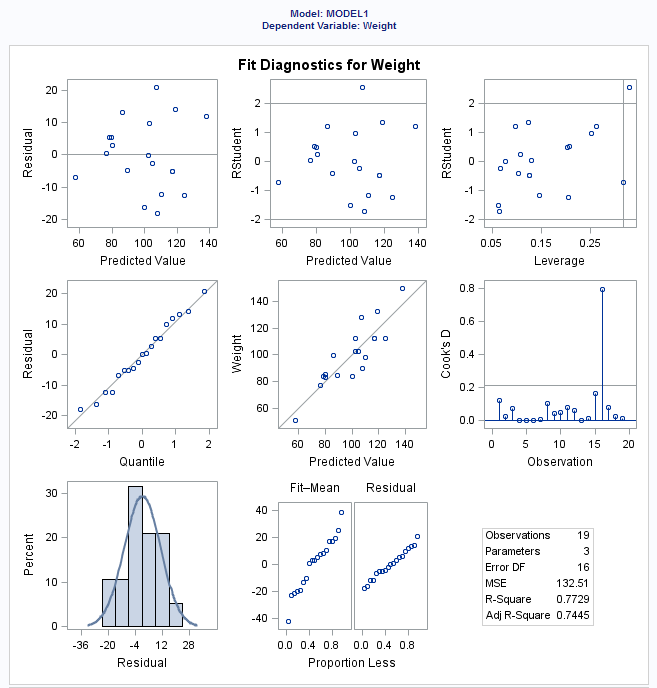
You can select the diagnostic, residual, and scatter plots to include in the results. By default, these plots are included in the results: plots of the fit diagnostics: residuals versus the predicted values studentized residuals versus the predicted values studentized residuals versus the leverage normal quantile plot of the residuals dependent variable versus the predicted values Cook’s D versus observation number histogram of residuals residual-fit plot, which includes side-by-side quantile plots of the centered fit and the residuals 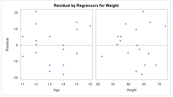residuals plot for each explanatory variable 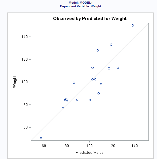a scatter plot of the observed values by predicted values You can also include these diagnostic plots: Rstudent statistic by predicted values plots studentized residuals by predicted values. If you select the Label extreme points option, observations with studentized residuals that lie outside the band between the reference lines are deemed outliers. DFFITS statistic by observations plots the DFFITS statistic by observation number. If you select the Label extreme points option, observations with a DFFITS statistic greater in magnitude than are deemed influential. The number of observations used is n, and the number of regressors is p. DFBETAS statistic by observation number for each explanatory variable produces panels of DFBETAS by observation number for the regressors in the model. You can view these plots as a panel or as individual plots. If you select the Label extreme points option, observations with a DFBETAS statistics greater in magnitude than $fraction 2 , over square root of n end fraction$ are deemed influential for that regressor. The number of observations used is n. You can also include these scatter plots: Fit plot for a single explanatory variable produces a scatter plot of the data overlaid with the regression line, confidence band, and prediction band for models that depend on at most one regressor. The intercept is excluded. When the number of points exceeds the value for the Maximum number of plot points option, a heat map is displayed instead of a scatter plot. Partial regression plots for each explanatory variable produces partial regression plots for each regressor. If you display these plots in a panel, there is a maximum of six regressors per panel.

Creating Output Data Sets

Option Name	Description
Output Data Sets
You can create two types of output data sets. By default, these data sets are saved in the Work library. Parameter estimates data set outputs a data set that contains parameter estimates and other model fit summary statistics. Any model selection statistics that you selected on the Methods tab are included in the parameter estimates. Observationwise statistics data set outputs a data set that contains sums of squares and cross-products.

Option Name

Description

Output Data Sets

You can create two types of output data sets. By default, these data sets are saved in the Work library.

Parameter estimates data set

outputs a data set that contains parameter estimates and other model fit summary statistics. Any model selection statistics that you selected on the Methods tab are included in the parameter estimates.

Observationwise statistics data set

outputs a data set that contains sums of squares and cross-products.