Setting Options

classifies the input binary response observations according to whether the predicted event probabilities are above or below the cut-point value z in the range. An observation is predicted as an event if the predicted event probability equals or exceeds z.

computes the partial correlation statistic 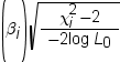for each parameter i, where X²_i is the Wald chi-square statistic for the parameter and log L₀ is the log-likelihood of the intercept-only model (Hilbe 2009). If X²_i < 2, the partial correlation is set to 0.

requests a generalized R square measure for the fitted model.

specifies whether to calculate the deviance and Pearson goodness-of-fit.

specifies the subpopulations on which the Pearson chi-square test statistic and the likelihood ratio chi-square test statistic (deviance) are calculated. Observations with common values in the given list of variables are regarded as coming from the same subpopulation. Variables in the list can be any variables in the input data set.

specifies whether to correct for overdispersion by using the Deviance or Pearson estimate.

performs the Hosmer and Lemeshow goodness-of-fit test (Hosmer and Lemeshow 2000) for the case of a binary response model. The subjects are divided into approximately 10 groups of approximately the same size based on the percentiles of the estimated probabilities. The discrepancies between the observed and expected number of observations in these groups are summarized by the Pearson chi-square statistic. This statistic is then compared to a chi-square distribution with t degrees of freedom, where t is the number of groups minus n. By default, n = 2. A small p-value suggests that the fitted model is not an adequate model.

specifies whether to compute and compare the least squares means of fixed effects.

specifies the effects that you want to compare. You specified these effects on the Model tab.

requests a multiple comparison adjustment for the p-values and confidence limits for the differences of the least squares means. Here are the valid methods: Bonferroni, Nelson, Scheffé, Sidak, and Tukey.

requests that a t type confidence interval be constructed for each of the least squares means with a confidence level of 1 – number. The value of number must be between 0 and 1. The default value is 0.05.

calculates the exact test for the intercept.

calculates exact tests of the parameters for the selected effects.

specifies the level of significance for confidence limits for the parameters or odds ratios.

You can calculate these parameter estimates:

displays the diagnostic measures for identifying influential observations. For each observation, the results include the sequence number of the observation, the values of the explanatory variables included in the final model, and the regression diagnostic measures developed by Pregibon (1981). You can specify whether to include the standardized and likelihood residuals in the results.

You can select whether to include plots in the results.

specifies the variable from the input data that contains the labels for the influence and ROC plots.

specifies the maximum number of points to include in the plots. By default, 5,000 points are shown.

specifies the optimization technique for estimating the regression parameters. The Fisher scoring and Newton-Raphson algorithms yield the same estimates, but the estimated covariance matrices are slightly different except when the Logit link function is specified for binary response data.

specifies the maximum number of iterations to perform. If convergence is not attained in a specified number of iterations, the displayed output and all output data sets created by the task contain results that are based on the last maximum likelihood iteration.