Example: Exploring the Sashelp.PriceData Data Set

To create this example:

In the Tasks section, expand the Forecasting folder, and then double-click Time Series Exploration. The user interface for the Time Series Exploration task opens.
On the Data tab, select the SASHELP.PRICEDATA data set.

Tip
If the data set is not available from the drop-down list, click . In the Choose a Table window, expand the library that contains the data set that you want to use. Select the data set for the example and click OK. The selected data set should now appear in the drop-down list.
Assign columns to these roles and specify these options:
1. To the Dependent variable role, assign the sale variable.
2. Expand the Additional Roles heading. To the Time ID role, assign the date variable. From the Interval drop-down list, select Quarter.
3. In the Transformations table, find the sale variable. From the Accumulation drop-down list, select Sum.
Click the Analyses tab, and select these series plots:
- Time Series
- Series histogram
- Seasonal cycles
To run the task, click .

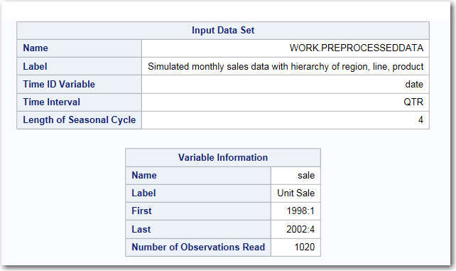
The first part of the results describes the input data set. This information shows the name and interval of the time ID variable and information about the dependent variable.

The time series plot suggests that there is a cyclical nature to sales for this product.

The histogram shows the distribution of sales for the series. Both a normal distribution and a kernel distribution are overlaid on the histogram.

The seasonal cycle plot shows that sales peak in Quarter 2 and are the lowest in Quarter 4.