Time Series Analysis for Multiple Dependent Variables :: SAS(R) Studio 3.5: Task Reference Guide

Example: Analyzing Sales and Cost Data

To create this example:

In the Tasks section, expand the Econometrics folder, and then double-click Time Series Analysis. The user interface for the Time Series Analysis task opens.
On the Data tab, select the SASHELP.PRDSALE data set.

Assign columns to these roles:

Role	Column Name
Dependent variables	ACTUAL PREDICT
Categorical variables	PRODUCT

To run the task, click .

Here is a subset of the results:

Simple Summary Statistics and Model Parameter Estimates

Assigning Data to Roles

To perform a time series analysis, you must assign an input data set. To filter the input data source, click Filter Icon

.

To perform a time series analysis with multiple dependent variables, you also must assign at least two variables to the Dependent variables role.

Role	Description
Roles
Dependent variables	specifies the dependent variables for the analysis.
Independent Variables
Continuous variables	specifies the independent variables for the model.
Categorical variables	specifies the classification variables to use in the analysis.
Time series ID	specifies the datetime values for the series. If you assign a SAS date or datetime variable to this role, the task automatically determines the time interval for these values. You can change this interval and also specify the multiplier, shift, and seasonal length. For more information about these options, see Understanding SAS Time Intervals. Note: This role is available only if you have multiple dependent variables.
Additional Roles
Group analysis by	enables you to obtain separate analyses of observations for each unique group.

Setting the Model Options

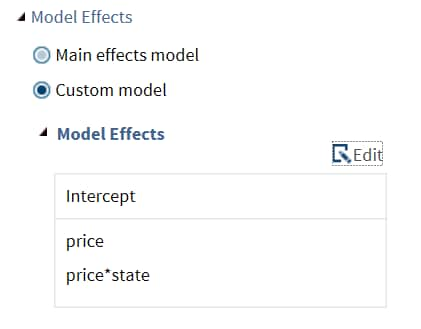
You can display the main effects model or create a custom model. To create a custom model, select the Custom Model option, and then click Edit. The Model Effects Builder opens. All continuous variables and categorical variables are listed in the Variables pane.

To create a main effect, select the variable in the Variables pane, and then click Add.
To create a crossed effect, select the variables in the Variables pane. (You can use Ctrl to select multiple variables.) Then click Cross.

When you finish, click OK. The effects that you specified now appear on the Model tab.

Here is an example of model effects on the Model tab.

Here are the remaining options on the Model tab.

Option Name	Description
Model Settings
Process Model
Automatically select process orders	removes insignificant autoregressive and moving average orders based on the value of the information criteria.
Autoregressive order (p), Maximum autoregressive order (p)	specifies the order of the autoregressive process.
Moving average order (q), Maximum average order (q)	specifies the order of the moving average process.
Exogenous variables lag (xlag)	specifies the lags for the exogenous variables.
GARCH Conditional Heteroscedasticity
ARCH process order (q)	specifies the order of the ARCH process to be fitted.
GARCH process order (p)	specifies the order of the GARCH process to be fitted. Note: This option is available only if you specify an ARCH process order greater than 0.
GARCH model representation	specifies the type of multivariate GARCH model representation. Here are the valid options: BEKK Constant conditional correlation Dynamic conditional correlation Note: This option is available only if you specify an ARCH process order greater than 0.
GARCH model type	specifies the subform type of GARCH model. Here are the valid options: Exponential GARCH Power GARCH Quadratic GARCH Threshold GARCH GARCH with no constraints Note: This option is available only if you select constant conditional correlation representation or the dynamic conditional correlation representation.
Vector Error Correction
Cointegration rank	specifies the cointegration rank of the cointegrated system. The rank of cointegration must be less than the number of dependent variables.
Select a normalization variable	specifies a dependent variable whose cointegrating vectors are normalized.

Setting the Options

Option Name	Description
Methods
Optimization method	specifies the optimization method to use. By default, no optimization method is used.
Maximum number of iterations	specifies the maximum number of iterations. You can use the default value or specify a custom value.
Statistics
You can include these statistics in the results: Dickey-Fuller unit root test Cointegration tests Estimated correlations of the parameter estimates Estimated covariances of the parameter estimates Residual diagnostics and model diagnostics Impulse response function Impulse response function related to exogenous (independent) variables Eigenvalues of the companion matrix associated with the AR characteristic function Yule-Walker estimates of the autoregressive model for the dependent variables
Plots
You can choose to include the default plots in the results, only selected plots, all of the plots, or none of the plots. You can also include these plots in the results: forecast plot impulse response function dependent variables and the one-step-ahead predicted values

Creating an Output Data Set

You can create these output data sets:

a data set that contains the actual values, forecast values, residuals, standard deviation of the forecasts, and the upper and lower confidence limits for the forecast
a data set of the parameter estimates
a data set of the residual diagnostics