Setting the Model Options
To use the Modeling and Forecasting task, you must
select a forecasting model type. You can choose from six model types:
random walk, moving average, exponential smoothing, ARIMA, ARIMAX,
and unobserved components.
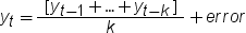
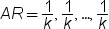
Moving Average
Exponential Smoothing
Exponential smoothing
is a forecasting technique that uses exponentially declining weights
to produce a weighted moving average of time series values. You can
choose from several forecasting models.
To create an exponential
smoothing model:
-
From the Forecasting model drop-down list, select the model that you want to use. You can choose from these models.
-
Simple (single) exponential smoothing, which is the default
-
Double (Brown) exponential smoothing
-
Linear (Holt) exponential smoothing
-
Damped trend exponential smoothing
-
Additive seasonal exponential smoothing
-
Multiplicative seasonal exponential smoothing
-
Winters multiplicative model
-
Winter additive model
-
ARIMA
When you create an Autoregressive
Integrated Moving Average (ARIMA) model, you can specify the autoregressive
and moving average polynomials of an ARIMA model.
To create an ARIMA
model:
-
Under the ARIMA heading, specify the autoregressive, differencing, and moving average orders for the ARIMA model.Here are the options for the simple ARIMA:
-
Autoregressive order (p) specifies the simple autoregressive order. You can specify an integer from 0 to 13. The default value is 0.
-
Differencing order (d) specifies the simple differencing order. You can specify an integer from 0 to 13. The default value is 0.
-
Moving average order (q) specifies the simple moving average. You can specify an integer from 0 to 13. The default value is 0.
Here are the options for the seasonal ARIMA:-
Autoregressive order (P) specifies the seasonal autoregressive order. You can specify an integer from 0 to 5. The default value is 0.
-
Differencing order (D) specifies the simple differencing order. You can specify an integer from 0 to 3. The default value is 0.
-
Moving average order (Q) specifies the simple moving average. You can specify an integer from 0 to 5. The default value is 0.
-
ARIMAX
When you create an Autoregressive
Integrated Moving Average (ARIMA) model, you can specify the autoregressive
and moving average polynomials of an ARIMA model. In an ARIMAX model,
you can also include independent variables in the model.
To create an ARIMAX
model:
-
Under the ARIMA heading, specify the autoregressive, differencing, and moving average orders for the ARIMA model.Here are the options for the simple ARIMA:
-
Autoregressive order (p) specifies the simple autoregressive order. You can specify an integer from 0 to 13. The default value is 0.
-
Differencing order (d) specifies the simple differencing order. You can specify an integer from 0 to 13. The default value is 0.
-
Moving average order (q) specifies the simple moving average. You can specify an integer from 0 to 13. The default value is 0.
Here are the options for the seasonal ARIMA:-
Autoregressive order (P) specifies the seasonal autoregressive order. You can specify an integer from 0 to 5. The default value is 0.
-
Differencing order (D) specifies the simple differencing order. You can specify an integer from 0 to 3. The default value is 0.
-
Moving average order (Q) specifies the simple moving average. You can specify an integer from 0 to 5. The default value is 0.
-
Unobserved Components
To create an unobserved
components model:
-
To include an irregular component, expand the Irregular Component heading and select the Include an irregular component check box. An irregular component is included by default.The irregular component corresponds to the overall random error in the model. The initial variance is the value used as the initial value during the parameter estimation process. To change this value, select Specify variance and enter a different value. To keep this value as your initial variance, select Fix variance value.
-
To include a trend component, expand the Trend Component heading. The level component and the slope component combine to define the trend component for the model. If you specify both a level and slope component, then a locally linear trend is obtained. If you omit the slope component, then a local level is used.
-
(Optional) To include a seasonal component, the season length must be greater than one. Expand the Seasonal Component heading and select the Include a seasonal component check box. Specify the type of seasonal component. A seasonal component can be one of two types: dummy or trigonometric. You can also specify whether to change the initial variance (which is 0 by default).
-
(Optional) To include a cycle component, expand the Cycle Component heading and select the Include a cycle component check box. You can specify these options:
-
To specify an initial cycle period to use during the parameter estimation process, select the Specify cycle period check box. Then specify the initial value in the box. This value must be an integer greater than 2. By default, the initial value is 3.
-
To specify an initial damping factor to use during the parameter estimation process, select the Specify damping factor check box, and then specify the initial value in the box. You can specify any value between 0 and 1 (excluding 0 but including 1). By default, the initial value is 0.01.
-
To specify an initial value for the disturbance variance parameter that the task uses during the parameter estimation process, select the Specify variance check box. Then specify the initial value in the box. This value must be greater than or equal to 0. By default, the initial value is 0.
-
Copyright © SAS Institute Inc. All rights reserved.