Introduction to Statistical Modeling with SAS/STAT Software
Analysis of Variance
![\[ \bY = \bX \tilde{\bbeta } + \left(\bY -\bX \tilde{\bbeta }\right) \]](images/statug_intromod0341.png)
holds for all vectors  , but only for the least squares solution is the residual
  orthogonal to the predicted value
  . Because of this orthogonality, the additive identity holds not only for the vectors themselves, but also for their lengths
(Pythagorean theorem):
. Because of this orthogonality, the additive identity holds not only for the vectors themselves, but also for their lengths
(Pythagorean theorem):
![\[ ||\bY ||^2 = ||\bX \widehat{\bbeta }||^2 + ||(\bY -\bX \widehat{\bbeta })||^2 \]](images/statug_intromod0362.png)
Note that 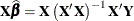 =
=  and note that
 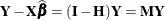 . The matrices
  and
and  play an important role in the theory of linear models and in statistical computations. Both
are projection matrices—that is, they are symmetric and idempotent. (An idempotent matrix
play an important role in the theory of linear models and in statistical computations. Both
are projection matrices—that is, they are symmetric and idempotent. (An idempotent matrix  is a square matrix that satisfies
  . The eigenvalues of an idempotent matrix take on the values 1 and 0 only.) The matrix projects onto the subspace of
  that is spanned by the columns of
  . The matrix
  projects onto the orthogonal complement of that space. Because of these properties you have
  ,
,  ,
,  ,
,  ,
,  .
.
The Pythagorean relationship now can be written in terms of  and as follows:
![\[ ||\bY ||^2 = \bY ’\bY = ||\mb{HY}||^2 + ||\mb{MY}||^2 = \bY ’\bH ’\bH \bY + \bY ’\bM ’\bM \bY = \bY ’\mb{HY} + \bY ’\mb{MY} \]](images/statug_intromod0376.png)
If  is deficient in rank and a generalized inverse is used to solve the normal equations, then you work instead with the projection
matrices
is deficient in rank and a generalized inverse is used to solve the normal equations, then you work instead with the projection
matrices 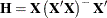 . Note that if
  is a generalized inverse of , then
  , and hence also and , are invariant to the choice of .
The matrix is sometimes referred to as the "hat" matrix because when you premultiply the vector of observations with , you produce the fitted values, which are commonly denoted by placing a "hat" over the  vector,
  .
.
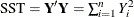
The term  is the uncorrected total sum of squares (
 ) of the linear model,
  is the error (residual) sum of squares (
 ), and
  is the uncorrected model sum of squares. This leads to the analysis of variance table shown in Table 3.2.
Table 3.2: Analysis of Variance with Uncorrected Sums of Squares
|
Source |
df |
Sum of Squares |
|---|---|---|
|
Model |
|
|
|
Residual |
|
|
|
|
||
|
Uncorr. Total |
n |
|


When the model contains an intercept term, then the analysis of variance is usually corrected for the mean, as shown in Table 3.3.
Table 3.3: Analysis of Variance with Corrected Sums of Squares
|
Source |
df |
Sum of Squares |
|---|---|---|
|
Model |
|
|
|
Residual |
|
|
|
|
||
|
Corrected Total |
|
|

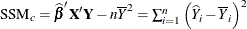


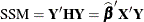
The coefficient of determination, also called the R-square statistic, measures the proportion of the total variation explained by the linear model. In models with intercept, it is defined as the ratio
![\[ R^2 = 1 - \frac{ \mr{SSR} }{ \mr{SST}_ c } = 1 - \frac{ \sum _{i=1}^ n \left(Y_ i - \widehat{Y}_ i\right)^2 }{ \sum _{i=1}^ n \left(Y_ i - \overline{Y} \right)^2 } \]](images/statug_intromod0395.png)
In models without intercept, the R-square statistic is a ratio of the uncorrected sums of squares
![\[ R^2 = 1 - \frac{ \mr{SSR} }{ \mr{SST} } = 1 - \frac{ \sum _{i=1}^ n \left(Y_ i - \widehat{Y}_ i\right)^2 }{ \sum _{i=1}^ n Y_ i^2 } \]](images/statug_intromod0396.png)