Introduction to Mixed Modeling Procedures
Linear Mixed Model
It is a defining characteristic of the class of linear mixed models (LMM), the class of generalized linear mixed models (GLMM), and the class of nonlinear mixed models (NLMM) that the random effects are normally distributed. In the linear mixed model, this also applies to the error term; furthermore, the errors and random effects are uncorrelated. The standard linear mixed model (LMM) is thus represented by the following assumptions:
![\begin{align*} \bY =& \, \, \bX \bbeta + \bZ \bgamma + \bepsilon \\ \bgamma \sim & \, \, N(\mb{0},\bG ) \\ \bepsilon \sim & \, \, N(\mb{0},\bR ) \\ \mr{Cov}[\bgamma ,\bepsilon ] =& \, \, \mb{0} \end{align*}](images/statug_intromix0007.png)
The matrices  and
and  are covariance matrices for the random effects and the random errors, respectively.
A G-side random effect in a linear mixed model is an element of
are covariance matrices for the random effects and the random errors, respectively.
A G-side random effect in a linear mixed model is an element of  , and its variance is expressed through an element in .
An R-side random variable is an element of
, and its variance is expressed through an element in .
An R-side random variable is an element of  , and its variance is an element of . The GLIMMIX, HPMIXED, and MIXED procedures express the and matrices in parametric form—that is, you structure the
covariance matrix, and its elements are expressed as functions of some parameters, known as the
covariance parameters of the mixed models. The NLMIXED procedure also parameterizes the covariance structure, but you accomplish this with programming
statements rather than with predefined syntax.
, and its variance is an element of . The GLIMMIX, HPMIXED, and MIXED procedures express the and matrices in parametric form—that is, you structure the
covariance matrix, and its elements are expressed as functions of some parameters, known as the
covariance parameters of the mixed models. The NLMIXED procedure also parameterizes the covariance structure, but you accomplish this with programming
statements rather than with predefined syntax.
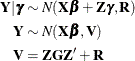
Since the right side of the model equation contains multiple random variables, the stochastic properties of  can be examined by conditioning on the random effects, or through the marginal
distribution. Because of the linearity of the G-side random effects and the normality of the random variables, the conditional
and the marginal distribution of the data are also normal with the following mean and variance matrices:
can be examined by conditioning on the random effects, or through the marginal
distribution. Because of the linearity of the G-side random effects and the normality of the random variables, the conditional
and the marginal distribution of the data are also normal with the following mean and variance matrices:
Parameter estimation in linear mixed models is based on likelihood or method-of-moment techniques. The default estimation method in PROC MIXED, and the only method available in PROC HPMIXED, is restricted (residual) maximum likelihood, a form of likelihood estimation that accounts for the parameters in the fixed-effects structure of the model to reduce the bias in the covariance parameter estimates. Moment-based estimation of the covariance parameters is available in the MIXED procedure through the METHOD= option in the PROC MIXED statement. The moment-based estimators are associated with sums of squares, expected mean squares (EMS), and the solution of EMS equations.
Parameter estimation by likelihood-based techniques in linear mixed models maximizes the marginal (restricted) log likelihood
of the data—that is, the log likelihood is formed from  . This is a model for with mean
  and covariance matrix
  , a correlated-error model. Such marginal models arise, for example, in the analysis of time series data, repeated measures, or spatial data, and are naturally subsumed into
the linear mixed model family. Furthermore, some mixed models have an equivalent formulation as a
correlated-error model, when both give rise to the same marginal mean and covariance matrix. For example, a mixed model with
a single variance component is identical to a correlated-error model with
compound-symmetric covariance structure, provided that the common correlation is positive.
, a correlated-error model. Such marginal models arise, for example, in the analysis of time series data, repeated measures, or spatial data, and are naturally subsumed into
the linear mixed model family. Furthermore, some mixed models have an equivalent formulation as a
correlated-error model, when both give rise to the same marginal mean and covariance matrix. For example, a mixed model with
a single variance component is identical to a correlated-error model with
compound-symmetric covariance structure, provided that the common correlation is positive.