Shared Concepts and Topics
Syntax: NLOPTIONS Statement
The NLOPTIONS statement provides you with syntax to control aspects of the nonlinear optimizations in the CALIS, GLIMMIX, HPMIXED, PHREG, SURVEYPHREG, and VARIOGRAM procedures.
-
NLOPTIONS <options>;
The nonlinear optimization options are described in alphabetical order after Table 19.28, which summarizes the options by category. The notation used in describing the options is generic in the sense that  denotes the
  vector of parameters for the optimization and
  is its ith element. The objective function being minimized, its gradient vector, and its
  Hessian matrix are denoted as
  ,
,  , and
, and  , respectively. The gradient with respect to the ith parameter is denoted as
  . Superscripts in parentheses denote the iteration count; for example,
  is the value of the objective function at iteration k. In the mixed model procedures, the parameter vector might consist of fixed effects only, covariance parameters only, or fixed effects and covariance parameters. In the CALIS
procedure, consists of all independent parameters that are defined in the models and in the PARAMETERS statement.
is the value of the objective function at iteration k. In the mixed model procedures, the parameter vector might consist of fixed effects only, covariance parameters only, or fixed effects and covariance parameters. In the CALIS
procedure, consists of all independent parameters that are defined in the models and in the PARAMETERS statement.
Table 19.28: Options to Control Aspects of the Optimization
|
Option |
Description |
|---|---|
|
Optimization |
|
|
Determines the type of Hessian scaling |
|
|
Specifies the start for approximated Hessian |
|
|
Specifies the line-search method |
|
|
Specifies the line-search precision |
|
|
Specifies the iteration number for update restart |
|
|
Determines the minimization technique |
|
|
Determines the update technique |
|
|
Termination Criteria |
|
|
Tunes an absolute function convergence criterion |
|
|
Tunes an absolute function difference convergence criterion |
|
|
Tunes the absolute gradient convergence criterion |
|
|
Tunes the absolute parameter convergence criterion |
|
|
Tunes the relative function convergence criterion |
|
|
Tunes another relative function convergence criterion |
|
|
Specifies the value used in the FCONV and GCONV criteria |
|
|
Tunes the relative gradient convergence criterion |
|
|
Tunes another relative gradient convergence criterion |
|
|
Specifies the maximum number of function calls |
|
|
Specifies the maximum number of iterations |
|
|
Specifies the upper limit for seconds of CPU time |
|
|
Specifies the minimum number of iterations |
|
|
Specifies the relative parameter convergence criterion |
|
|
Specifies the value used in the XCONV criterion |
|
|
Step Length |
|
|
Dampens steps in a line search |
|
|
Specifies the initial trust region radius |
|
|
Specifies the maximum trust region radius |
|
|
Printed Output |
|
|
Displays (almost) all printed output |
|
|
Displays optimization history |
|
|
Suppresses all printed output |
|
|
Covariance Matrix Tolerances |
|
|
Specifies the absolute singularity for inertia |
|
|
Specifies the relative M singularity for inertia |
|
|
Specifies the relative V singularity for inertia |
|
|
Constraint Specifications |
|
|
Specifies the range for active constraints |
|
|
Specifies the LM tolerance for deactivating |
|
|
Specifies the tolerance for dependent constraints |
|
|
Remote Monitoring |
|
|
Specifies the fileref for remote monitoring |
|
-
ABSCONV=r
ABSTOL=r -
specifies an absolute function convergence criterion: for minimization, termination requires
 . The default value of r is the negative square root of the largest double-precision value, which serves only as a protection against overflows.
-
ABSFCONV=r <n>
ABSFTOL=r<n> -
specifies an absolute function difference convergence criterion:
-
For all techniques except NMSIMP (specified by the TECHNIQUE= option), termination requires a small change of the function value in successive iterations,
![\[ |f(\bpsi ^{(k-1)}) - f(\bpsi ^{(k)})| \leq \Argument{r} \]](images/statug_introcom0175.png)
-
The same formula is used for the NMSIMP technique, but
 is defined as the vertex with the lowest function value, and
  is defined as the vertex with the highest function value in the simplex.
The default value is r = 0. The optional integer value n specifies the number of successive iterations for which the criterion must be satisfied before the process can be terminated.
-
-
ABSGCONV=r <n>
ABSGTOL=r<n> -
specifies an absolute gradient convergence criterion:
-
For all techniques except NMSIMP (specified by the TECHNIQUE= option), termination requires the maximum absolute gradient element to be small:
![\[ \max _ j |g_ j(\bpsi ^{(k)})| \leq \Argument{r} \]](images/statug_introcom0178.png)
-
This criterion is not used by the NMSIMP technique.
The default value is r = 1E–5. The optional integer value n specifies the number of successive iterations for which the criterion must be satisfied before the process can be terminated.
-
-
ABSXCONV=r <n>
ABSXTOL=r<n> -
specifies an absolute parameter convergence criterion:
-
For all techniques except NMSIMP, termination requires a small Euclidean distance between successive parameter vectors,
![\[ \parallel \bpsi ^{(k)} - \bpsi ^{(k-1)} \parallel _2 \leq \Argument{r} \]](images/statug_introcom0179.png)
-
For the NMSIMP technique, termination requires either a small length
 of the vertices of a restart simplex,
![\[ \alpha ^{(k)} \leq \Argument{r} \]](images/statug_introcom0181.png)
or a small simplex size,
![\[ \delta ^{(k)} \leq \Argument{r} \]](images/statug_introcom0182.png)
where the simplex size
 is defined as the L1 distance from the simplex vertex
  with the smallest function value to the other p simplex points
  :
:
![\[ \delta ^{(k)} = \sum _{\bpsi _ l \neq y} \parallel \bpsi _ l^{(k)} - \bxi ^{(k)}\parallel _1 \]](images/statug_introcom0186.png)
The default is r = 1E–8 for the NMSIMP technique and r = 0 otherwise. The optional integer value n specifies the number of successive iterations for which the criterion must be satisfied before the process can terminate.
-
-
ASINGULAR=r
ASING=r -
specifies an absolute singularity criterion for the computation of the inertia (number of positive, negative, and zero eigenvalues) of the Hessian and its projected forms. The default value is the square root of the smallest positive double-precision value.
- DAMPSTEP<=r>
-
specifies that the initial step length value
 for each
line search (used by the QUANEW, CONGRA, or NEWRAP technique) cannot be larger than r times the step length value used in the former iteration. If the DAMPSTEP option is specified but r is not specified, the default is r = 2. The DAMPSTEP= option can prevent the line-search algorithm from repeatedly stepping into regions where some objective
functions are difficult to compute or where they could lead to floating-point overflows during the computation of objective
functions and their derivatives. The DAMPSTEP= option can save time-consuming function calls during the line searches of objective
functions that result in very small steps.
for each
line search (used by the QUANEW, CONGRA, or NEWRAP technique) cannot be larger than r times the step length value used in the former iteration. If the DAMPSTEP option is specified but r is not specified, the default is r = 2. The DAMPSTEP= option can prevent the line-search algorithm from repeatedly stepping into regions where some objective
functions are difficult to compute or where they could lead to floating-point overflows during the computation of objective
functions and their derivatives. The DAMPSTEP= option can save time-consuming function calls during the line searches of objective
functions that result in very small steps.
-
FCONV=r<n>
FTOL=r<n> -
specifies a relative function convergence criterion:
-
For all techniques except NMSIMP, termination requires a small relative change of the function value in successive iterations,
![\[ \frac{|f(\bpsi ^{(k)}) - f(\bpsi ^{(k-1)})|}{\max (|f(\bpsi ^{(k-1)})|,\mr{FSIZE}) } \leq \Argument{r} \]](images/statug_introcom0188.png)
where FSIZE is defined by the FSIZE= option.
-
The same formula is used for the NMSIMP technique, but
 is defined as the vertex with the lowest function value and is defined as the vertex with the highest function value in the simplex.
The default is r
 , where FDIGITS is by default
  and
and  is the machine precision. Some procedures, such as the GLIMMIX procedure, enable you to change the value with the FDIGITS=
option in the PROC statement. The optional integer value n specifies the number of successive iterations for which the criterion must be satisfied before the process can terminate.
is the machine precision. Some procedures, such as the GLIMMIX procedure, enable you to change the value with the FDIGITS=
option in the PROC statement. The optional integer value n specifies the number of successive iterations for which the criterion must be satisfied before the process can terminate.
-
-
FCONV2=r<n>
FTOL2=r<n> -
specifies a second function convergence criterion:
-
For all techniques except NMSIMP, termination requires a small predicted reduction,
![\[ \mi{df}^{(k)} \approx f(\bpsi ^{(k)}) - f(\bpsi ^{(k)} + \mb{s}^{(k)}) \]](images/statug_introcom0192.png)
of the objective function. The predicted reduction
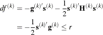
is computed by approximating the objective function f by the first two terms of the Taylor series and substituting the Newton step,
![\[ \mb{s}^{(k)} = - [\mb{H}^{(k)}]^{-1} \mb{g}^{(k)} \]](images/statug_introcom0194.png)
-
For the NMSIMP technique, termination requires a small standard deviation of the function values of the
 simplex vertices
  ,
,  ,
,
![\[ \sqrt { \frac{1}{n+1} \sum _ l \left[ f(\bpsi _ l^{(k)}) - \overline{f}(\bpsi ^{(k)}) \right]^2 } \leq \Argument{r} \]](images/statug_introcom0198.png)
where
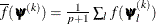 . If there are
  boundary constraints active at , the mean and standard deviation are computed only for the
  unconstrained vertices.
The default value is r = 1E–6 for the NMSIMP technique and r= 0 otherwise. The optional integer value n specifies the number of successive iterations for which the criterion must be satisfied before the process can terminate.
-
- FSIZE=r
-
specifies the FSIZE parameter of the relative function and relative gradient termination criteria. The default value is r = 0. For more details, see the FCONV= and GCONV= options.
-
GCONV=r<n>
GTOL=r<n> -
specifies a relative gradient convergence criterion:
-
For all techniques except CONGRA and NMSIMP, termination requires that the normalized predicted function reduction be small,
![\[ \frac{\mb{g}(\bpsi ^{(k)})^\prime [\bH ^{(k)}]^{-1} \mb{g}(\bpsi ^{(k)})}{\max (|f(\bpsi ^{(k)})|,\mr{FSIZE}) } \leq \Argument{r} \]](images/statug_introcom0202.png)
where FSIZE is defined by the FSIZE= option. For the CONGRA technique (where a reliable Hessian estimate
 is not available), the following criterion is used:
![\[ \frac{\parallel \mb{g}(\bpsi ^{(k)}) \parallel _2^2 \quad \parallel \mb{s}(\bpsi ^{(k)}) \parallel _2}{\parallel \mb{g}(\bpsi ^{(k)}) - \mb{g}(\bpsi ^{(k-1)}) \parallel _2 \max (|f(\bpsi ^{(k)})|,\mr{FSIZE}) } \leq \Argument{r} \]](images/statug_introcom0204.png)
-
This criterion is not used by the NMSIMP technique.
The default value is r = 1E–8. The optional integer value n specifies the number of successive iterations for which the criterion must be satisfied before the process can terminate.
-
-
GCONV2=r<n>
GTOL2=r<n> -
specifies another relative gradient convergence criterion:
-
For least squares problems and the TRUREG, LEVMAR, NRRIDG, and NEWRAP techniques, the following criterion of Browne (1982) is used:
![\[ \max _ j \frac{|\mb{g}_ j(\bpsi ^{(k)})|}{\sqrt {f(\bpsi ^{(k)}) \bH _{j,j}^{(k)}}} \leq \Argument{r} \]](images/statug_introcom0205.png)
-
This criterion is not used by the other techniques.
The default value is r = 0. The optional integer value n specifies the number of successive iterations for which the criterion must be satisfied before the process can terminate.
-
-
HESCAL=0 | 1 | 2 | 3
HS=0 | 1 | 2 | 3 -
specifies the scaling version of the Hessian (or crossproduct Jacobian) matrix used in NRRIDG, TRUREG, LEVMAR, NEWRAP, or DBLDOG optimization.
If HS is not equal to 0, the first iteration and each restart iteration set the diagonal scaling matrix
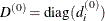 :
:
![\[ d_ i^{(0)} = \sqrt {\max (|H^{(0)}_{i,i}|,\epsilon )} \]](images/statug_introcom0207.png)
where
 are the diagonal elements of the Hessian (or crossproduct Jacobian). In every other iteration, the diagonal scaling matrix
is updated depending on the HS option:
are the diagonal elements of the Hessian (or crossproduct Jacobian). In every other iteration, the diagonal scaling matrix
is updated depending on the HS option:
In each scaling update,
is the relative machine precision. The default value is HS=0. Scaling of the Hessian can be time-consuming in the case where
general linear constraints are active.
-
INHESSIAN<=r>
INHESS<=r> -
specifies how the initial estimate of the approximate Hessian is defined for the quasi-Newton techniques QUANEW and DBLDOG. There are two alternatives:
-
If you do not use the r specification, the initial estimate of the approximate Hessian is set to the Hessian at
 .
.
-
If you do use the r specification, the initial estimate of the approximate Hessian is set to the multiple of the identity matrix r
 .
.
By default (if you do not specify the option INHESSIAN=r), the initial estimate of the approximate Hessian is set to the multiple of the identity matrix r
, where the scalar r is computed from the magnitude of the initial gradient.
-
-
INSTEP=r
SALPHA=r
RADIUS=r -
reduces the length of the first trial step during the line search of the first iterations. For highly nonlinear objective functions, such as the EXP function, the default initial radius of the trust-region algorithm TRUREG or DBLDOG or the default step length of the line-search algorithms can result in arithmetic overflows. If this occurs, you should specify decreasing values of 0 < r < 1 such as INSTEP=1E–1, INSTEP=1E–2, INSTEP=1E–4, and so on, until the iteration starts successfully.
-
For trust-region algorithms (TRUREG or DBLDOG), the INSTEP= option specifies a factor r > 0 for the initial radius
 of the trust region. The default initial trust-region radius is the length of the scaled gradient. This step corresponds
to the default radius factor of r = 1.
of the trust region. The default initial trust-region radius is the length of the scaled gradient. This step corresponds
to the default radius factor of r = 1.
-
For line-search algorithms (NEWRAP, CONGRA, or QUANEW), the INSTEP= option specifies an upper bound for the initial step length for the line search during the first five iterations. The default initial step length is r = 1.
-
For the Nelder-Mead simplex algorithm, by using TECH=NMSIMP, the INSTEP=r option defines the size of the start simplex.
-
-
LCDEACT=r
LCD=r -
specifies a threshold r for the Lagrange multiplier that determines whether an active inequality constraint remains active or can be deactivated. For maximization, r must be greater than zero; for minimization, r must be smaller than zero. An active inequality constraint can be deactivated only if its Lagrange multiplier is less than the threshold value. The default value is
![\[ \Argument{r} = \pm \min (0.01, \max (0.1 \times \mr{ABSGCONV}, 0.001 \times \mr{gmax}^{(k)})) \]](images/statug_introcom0216.png)
where "+" is for maximization, "–" is for minimization, ABSGCONV is the value of the absolute gradient criterion, and
 is the maximum absolute element of the gradient or the projected gradient.
-
LCEPSILON=r
LCEPS=r
LCE=r -
specifies the range r for active and violated boundary constraints, where r
 0. If the point satisfies the following condition, the constraint i is recognized as an active constraint:
![\[ | \sum _{j=1}^ k a_{ij}\psi _ j^{(k)} - b_ i | \leq \Argument{r} \times \left(|b_ i|+1\right) \]](images/statug_introcom0219.png)
Otherwise, the constraint i is either an inactive inequality or a violated inequality or equality constraint. The default value is r = 1E–8. During the optimization process, the introduction of rounding errors can force the optimization to increase the value of r by a factor of
 for some k > 0. If this happens, it is indicated by a message displayed in the log.
-
LCSINGULAR=r
LCSING=r
LCS=r -
specifies a criterion r, where r
0, that is used in the update
of the QR decomposition and that determines whether an active constraint is linearly dependent on a set of other active constraints.
The default value is r = 1E–8. The larger r becomes, the more the active constraints are recognized as being linearly dependent. If the value of r is larger than 0.1, it is reset to 0.1.
-
LINESEARCH=i
LIS=i -
specifies the line-search method for the CONGRA, QUANEW, and NEWRAP optimization techniques. See Fletcher (1987) for an introduction to line-search techniques. The value of i can be
 as follows. The default is LIS=2.
- 1
-
specifies a line-search method that needs the same number of function and gradient calls for cubic interpolation and cubic extrapolation; this method is similar to one used by the Harwell subroutine library.
- 2
-
specifies a line-search method that needs more function than gradient calls for quadratic and cubic interpolation and cubic extrapolation; this method is implemented as shown in Fletcher (1987) and can be modified to an exact line search by using the LSPRECISION= option. This is the default.
- 3
-
specifies a line-search method that needs the same number of function and gradient calls for cubic interpolation and cubic extrapolation; this method is implemented as shown in Fletcher (1987) and can be modified to an exact line search by using the LSPRECISION= option.
- 4
-
specifies a line-search method that needs the same number of function and gradient calls for stepwise extrapolation and cubic interpolation.
- 5
-
specifies a line-search method that is a modified version of LIS=4.
- 6
-
specifies a golden-section line search (Polak 1971), which uses only function values for linear approximation.
- 7
-
specifies a bisection line search (Polak 1971), which uses only function values for linear approximation.
- 8
-
specifies the Armijo line-search technique (Polak 1971), which uses only function values for linear approximation.
-
LSPRECISION=r
LSP=r -
specifies the degree of accuracy that should be obtained by the line-search algorithms LIS= 2 and LIS= 3. Usually an imprecise line search is inexpensive and successful. For more difficult optimization problems, a more precise and expensive line search might be necessary (Fletcher 1987). The LIS=2 line-search method (which is the default for the NEWRAP, QUANEW, and CONGRA techniques) and the LIS=3 line-search method approach exact line search for small LSPRECISION= values. If you have numerical problems, try to decrease the LSPRECISION= value to obtain a more precise line search. The default values are shown in Table 19.29.
Table 19.29: Default Values for Line-Search Precision
TECH=
UPDATE=
LSP Default
QUANEW
DBFGS, BFGS
r = 0.4
QUANEW
DDFP, DFP
r = 0.06
CONGRA
All
r = 0.1
NEWRAP
No update
r = 0.9
For more details, see Fletcher (1987).
-
MAXFUNC=i
MAXFU=i -
specifies the maximum number i of function calls in the optimization process. The default values are as follows:
-
125 for the TRUREG, NRRIDG, NEWRAP, and LEVMAR techniques
-
500 for the QUANEW and DBLDOG techniques
-
1000 for the CONGRA technique
-
3000 for the NMSIMP technique
Optimization can terminate only after completing a full iteration. Therefore, the number of function calls that are actually performed can exceed the number that is specified by the MAXFUNC= option.
-
-
MAXITER=i
MAXIT=i -
specifies the maximum number i of iterations in the optimization process. The default values are as follows:
-
50 for the TRUREG, NRRIDG, NEWRAP, and LEVMAR techniques
-
200 for the QUANEW and DBLDOG techniques
-
400 for the CONGRA technique
-
1000 for the NMSIMP technique
These default values are also valid when i is specified as a missing value.
-
- MAXSTEP=r<n>
-
specifies an upper bound for the step length of the line-search algorithms during the first n iterations. By default, r is the largest double-precision value and n is the largest integer available. Setting this option can improve the speed of convergence for the CONGRA, QUANEW, and NEWRAP techniques.
- MAXTIME=r
-
specifies an upper limit of r seconds of CPU time for the optimization process. The time specified by the MAXTIME= option is checked only once at the end of each iteration. Therefore, the actual running time can be much longer than that specified by the MAXTIME= option. The actual running time includes the rest of the time needed to finish the iteration and the time needed to generate the output of the results. By default, CPU time is not limited.
-
MINITER=i
MINIT=i -
specifies the minimum number of iterations. The default value is 0. If you request more iterations than are actually needed for convergence to a stationary point, the optimization algorithms can behave strangely. For example, the effect of rounding errors can prevent the algorithm from continuing for the required number of iterations.
-
MSINGULAR=r
MSING=r -
specifies a relative singularity criterion r, where r > 0, for the computation of the inertia (number of positive, negative, and zero eigenvalues) of the Hessian and its projected forms. The default value is 1E–12.
- NOPRINT
-
suppresses output that is related to optimization, such as the iteration history. This option, along with all NLOPTIONS statement options for displayed output, are ignored by the GLIMMIX and HPMIXED procedures.
- PALL
-
displays all optional output for optimization. This option is supported only by the CALIS and SURVEYPHREG procedures.
-
PHISTORY
PHIST -
displays the optimization history. The PHISTORY option is implied if the PALL option is specified. The PHISTORY option is supported only by the CALIS and SURVEYPHREG procedures.
-
RESTART=i
REST=i -
specifies that the QUANEW or CONGRA technique is restarted with a steepest search direction after at most i iterations, where i > 0. Default values are as follows:
-
SINGULAR=r
SING=r -
specifies the singularity criterion r, 0
 r 1, that is
used for the inversion of the Hessian matrix. The default value is 1E–8.
r 1, that is
used for the inversion of the Hessian matrix. The default value is 1E–8.
- SOCKET=fileref
-
specifies the fileref that contains the information needed for remote monitoring.
-
TECHNIQUE=value
TECH=value
OMETHOD=value
OM=value -
specifies the optimization technique. You can find additional information about choosing an optimization technique in the section Choosing an Optimization Algorithm. Valid values for the TECHNIQUE= option are as follows:
-
CONGRA performs a conjugate-gradient optimization, which can be more precisely specified with the UPDATE= option and modified with the LINESEARCH= option. When you specify this option, UPDATE= PB by default.
-
DBLDOG performs a version of double-dogleg optimization, which can be more precisely specified with the UPDATE= option. When you specify this option, UPDATE= DBFGS by default.
-
LEVMAR performs a highly stable, but for large problems memory- and time-consuming, Levenberg-Marquardt optimization technique, a slightly improved variant of the Moré (1978) implementation. You can also specify this technique with the alias LM or MARQUARDT. In the CALIS procedure, this is the default optimization technique if there are fewer than 40 parameters to estimate. The GLIMMIX and HPMIXED procedures do not support this optimization technique.
-
NMSIMP performs a Nelder-Mead simplex optimization. The CALIS procedure does not support this optimization technique.
-
NONE does not perform any optimization. This option can be used for the following:
-
to perform a grid search without optimization
-
to compute estimates and predictions that cannot be obtained efficiently with any of the optimization techniques
-
to obtain inferences for known values of the covariance parameters
-
-
NEWRAP performs a Newton-Raphson optimization that combines a line-search algorithm with ridging. The line-search algorithm LIS= 2 is the default method.
-
NRRIDG performs a Newton-Raphson optimization with ridging. This is the default optimization technique in the SURVEYPHREG procedure.
-
QUANEW performs a quasi-Newton optimization, which can be defined more precisely with the UPDATE= option and modified with the LINESEARCH= option.
-
TRUREG performs a trust-region optimization.
-
-
UPDATE=method
UPD=method -
specifies the update method for the quasi-Newton, double-dogleg, or conjugate-gradient optimization technique. Not every update method can be used with each optimizer.
The following are the valid methods for the UPDATE= option:
-
BFGS performs the original Broyden, Fletcher, Goldfarb, and Shanno (BFGS) update of the inverse Hessian matrix.
-
DBFGS performs the dual BFGS update of the Cholesky factor of the Hessian matrix. This is the default update method.
-
DDFP performs the dual Davidon, Fletcher, and Powell (DFP) update of the Cholesky factor of the Hessian matrix.
-
DFP performs the original DFP update of the inverse Hessian matrix.
-
PB performs the automatic restart update method of Powell (1977) and Beale (1972).
-
FR performs the Fletcher-Reeves update (Fletcher 1987).
-
PR performs the Polak-Ribiere update (Fletcher 1987).
-
CD performs a conjugate-descent update of Fletcher (1987).
-
-
VERSION=1 | 2
VS=1 | 2 -
specifies the version of the quasi-Newton optimization technique with nonlinear constraints.
The default is VERSION=2.
-
VSINGULAR=r
VSING=r -
specifies a relative singularity criterion r, where r > 0, for the computation of the inertia (number of positive, negative, and zero eigenvalues) of the Hessian and its projected forms. The default value is r = 1E–8.
-
XCONV=r<n>
XTOL=r<n> -
specifies the relative parameter convergence criterion:
-
For all techniques except NMSIMP, termination requires a small relative parameter change in subsequent iterations:
![\[ \frac{\max _ j |\psi _ j^{(k)} - \psi _ j^{(k-1)}| }{\max (|\psi _ j^{(k)}|,|\psi _ j^{(k-1)}|,\mbox{XSIZE})} \leq \Argument{r} \]](images/statug_introcom0226.png)
-
For the NMSIMP technique, the same formula is used, but
 is defined as the vertex with the lowest function value and
  is defined as the vertex with the highest function value in the simplex.
The default value is r = 1E–8 for the NMSIMP technique and r = 0 otherwise. The optional integer value n specifies the number of successive iterations for which the criterion must be satisfied before the process can be terminated.
-
- XSIZE=r
-
specifies the XSIZE parameter r of the relative parameter termination criterion, where r
 0. The default value is r = 0. For more details, see the XCONV=
option.
0. The default value is r = 0. For more details, see the XCONV=
option.
![\[ d_ i^{(k+1)} = \max \left[ d_ i^{(k)},\sqrt {\max (|H^{(k)}_{i,i}|, \epsilon )} \right] \]](images/statug_introcom0209.png)
![\[ d_ i^{(k+1)} = \max \left[ 0.6 * d_ i^{(k)}, \sqrt {\max (|H^{(k)}_{i,i}|,\epsilon )} \right] \]](images/statug_introcom0210.png)

![\[ d_ i^{(k+1)} = \sqrt {\max (|H^{(k)}_{i,i}|,\epsilon )} \]](images/statug_introcom0212.png)


