The HPFMM Procedure

Model Options
- ALPHA=number
-
requests that confidence intervals be constructed for each of the parameters with confidence level
 . The value of number must be between 0 and 1; the default is 0.05.
- CL
-
requests that confidence limits be constructed for each of the parameter estimates. The confidence level is 0.95 by default; this can be changed with the ALPHA= option.
-
DISTRIBUTION=keyword
DIST=keyword -
specifies the probability distribution for a mixture component.
If you specify the DIST= option and you do not specify a link function with the LINK= option, a default link function is chosen according to Table 51.5. If you do not specify a distribution, the HPFMM procedure defaults to the normal distribution for continuous response variables and to the binary distribution for classification or character variables, unless the events/trial syntax is used in the MODEL statement. If you choose the events/trial syntax, the HPFMM procedure defaults to the binomial distribution.
Table 51.5 lists keywords that you can specify for the DISTRIBUTION= option and the corresponding default link functions. For generalized linear models with these distributions, you can find expressions for the log-likelihood functions in the section Log-Likelihood Functions for Response Distributions.
Table 51.5: Keyword Values of the DIST= Option
Default Link
keyword
Alias
Distribution
Function
BETA
Beta
Logit
BETABINOMIAL
BETABIN
Beta-binomial
Logit
BINARY
BERNOULLI
Binary
Logit
BINOMIAL
BIN
Binomial
Logit
BINOMCLUSTER
BINOMCLUS
Binomial cluster
Logit
CONSTANT <(c)>
DEGENERATE <(c)>
Degenerate
N/A
EXPONENTIAL
EXPO
Exponential
Log
FOLDEDNORMAL
FNORMAL
Folded normal
Identity
GAMMA
GAM
Gamma
Log
GAUSSIAN
NORMAL
Normal
Identity
GENPOISSON
GPOISSON
Generalized Poisson
Log
GEOMETRIC
GEOM
Geometric
Log
INVGAUSS
IGAUSSIAN, IG
Inverse Gaussian
Inverse squared
(power(–2))
LOGNORMAL
LOGN
Lognormal
Identity
NEGBINOMIAL
NEGBIN, NB
Negative binomial
Log
POISSON
POI
Poisson
Log
T <(
 )>
)>
STUDENT <(
)>
t
Identity
TRUNCEXPO <(a,b)>
TEXPO <(a,b)>
Truncated exponential
Log
TRUNCLOGN <(a,b)>
TLOGN <(a,b)>
Lognormal
Identity
TRUNCNEGBIN
TNEGBIN, TNB
Negative binomial
Log
TRUNCNORMAL <(a,b)>
TNORMAL <(a,b)>
Truncated normal
Identity
TRUNCPOISSON
TPOISSON, TPOI
Truncated Poisson
Log
UNIFORM <(a,b)>
UNIF <(a,b)>
Uniform
N/A
WEIBULL
Weibull
Log
Note that the PROC HPFMM default link for the gamma or exponential distribution is not the canonical link (the reciprocal link).
The binomial cluster model is a two-component model described in Morel and Nagaraj (1993); Morel and Neerchal (1997); Neerchal and Morel (1998). See Example 51.1 for an application of the binomial cluster model in a teratological experiment.
If the events/trials syntax is used, the default distribution is the binomial and only the following choices are available: DIST=BINOMIAL, DIST=BETABINOMIAL, and DIST=BINOMCLUSTER. The trials variable is ignored for all other distributions. This enables you to fit models in which some components have a binomial or binomial-like distribution. For example, suppose that variable
nis a binomial denominator and variablelognis its logarithm. Then the following statements model a two-component mixture of a binomial and Poisson count model:model y/n = ; model + / dist=Poisson offset=logn;
The OFFSET= option is used in the second MODEL statement to specify that the Poisson counts refer to different base counts, since the trial variable n is ignored in the second model.
If DIST=BINOMIAL is specified without the events/trials syntax, then n=1 is used for the default number of trials.
DIST=TRUNCNEGBIN and DIST=TRUNCPOISSON are zero-truncated versions of DIST=NEGBINOMIAL and DIST=POISSON, respectively—that is, only the value of 0 is excluded from the support.
For DIST=TRUNCEXPO, DIST=TRUNCLOGN, and DIST=TRUNCNORMAL, you must specify the lower (a) and upper (b) truncation points of the distribution. For example:
-
DIST=TRUNCEXPO<(a,b)>
-
DIST=TRUNCLOGN<(a,b)>
-
DIST=TRUNCNORMAL<(a,b)>
Each of these distributions is the conditional version of its corresponding nontruncated distribution that is confined to the support
![$[a, b]$](images/statug_hpfmm0118.png) (inclusive). You can specify a missing value (.) for either a or b to truncate only on the other side; that is, a=. indicates a right-truncated distribution, and b=. indicates a left-truncated distribution.
(inclusive). You can specify a missing value (.) for either a or b to truncate only on the other side; that is, a=. indicates a right-truncated distribution, and b=. indicates a left-truncated distribution.
For several distribution specifications you can provide additional optional parameters to further define the distribution. These optional parameters are listed in the following:
- CONSTANT<(c)>
-
The number c specifies the value where the mass is concentrated. The default is DIST=CONSTANT(0), so you can add zero-inflation to any model by adding a MODEL statement with DIST=CONSTANT.
- T<()>
-
The number
specifies the degrees of freedom for the (shifted) t distribution. The default is DIST=T(3); this leads to a heavy-tailed distribution for which the variance is defined. See
the section Log-Likelihood Functions for Response Distributions for the density function of the shifted  distribution.
- UNIFORM<(a,b)>
-
The values a and b define the support of the uniform distribution, a < b. By default, a = 0 and b = 1.
-
- EQUATE=MEAN | SCALE | NONE | EFFECTS(effect-list)
-
specifies simple sets of parameter constraints across the components in a MODEL statement; the default is EQUATE=NONE. This option is available only for maximum likelihood estimation. If you specify EQUATE=MEAN, the parameters that determine the mean are reduced to a single set that is applicable to all components in the MODEL statement. If you specify EQUATE=SCALE, a single parameter represents the common scale for all components in the MODEL statement. The EFFECTS option enables you to force the parameters for the chosen model effects to be equal across components; however, the number of parameters is unaffected.
For example, the following statements fit a two-component multiple regression model in which the coefficients for variable
logdvary by component and the intercepts and coefficients for variabledoseare the same for the two components:proc hpfmm; model num = dose logd / equate=effects(int dose) k=2; run;
To fix all coefficients across the two components, you can write the MODEL statement as
model num = dose logd / equate=effects(int dose logd) k=2;
or
model num = dose logd / equate=mean k=2;
If you restrict all parameters in a k-component MODEL statement to be equal, the HPFMM procedure reduces the model to k=1.
-
K=n
NUMBER=n -
specifies the number of components the MODEL statement contributes to the overall mixture. For the binomial cluster model, this option is not available, since this model is a two-component model by definition.
- KMAX=n
-
specifies the maximum number of components the MODEL statement contributes to the overall mixture.
If the maximum number of components in the mixture, as determined by all KMAX= options, is larger than the minimum number of components, the HPFMM procedure fits all possible models and displays summary fit information for the sequence of evaluated models. The "best" model according to the CRITERION= option in the PROC HPFMM statement is then chosen, and the remaining output and analyses performed by PROC HPFMM pertain to this "best" model.
When you use MCMC methods to estimate the parameters of a mixture, you need to ensure that the chain for a given value of k has converged; otherwise, comparisons among models that have varying numbers of components might not be meaningful. You can use the FITDETAILS option to display summary and diagnostic information for the MCMC chains from each model.
If you specify the KMIN= option but not the KMAX= option, then the default value for the KMAX= option is the value of the KMIN= option (unless KMIN= 0, in which case the KMAX= option is set to 1).
- KMIN=n
-
specifies the minimum number of components that the MODEL statement contributes to the overall mixture. When you use MCMC methods to estimate the parameters of a mixture, you need to ensure that the chain for a given value of k has converged; otherwise, comparisons among models that have varying numbers of components might not be meaningful.
- KRESTART
-
requests that the starting values for each analysis (that is, for each unique number of components as determined by the KMIN= and KMAX= options) be determined separately, in the same way as if no other analyses were performed. If you do not specify the KRESTART option, then the starting values for each analysis are based on results from the previous analysis with one less component.
- LABEL=’label’
-
specifies an optional label for the model that is used to identify the model in printed output, on graphics, and in data sets created from ODS tables.
- LINK=keyword
-
specifies the link function in the model. The keywords and expressions for the associated link functions are shown in Table 51.6.
Table 51.6: Link Functions in MODEL Statement of the HPFMM Procedure
Link
LINK=
Alias
Function

CLOGLOG
CLL
Complementary log-log
IDENTITY
ID
Identity

LOG
Log

LOGIT
Logit

LOGLOG
Log-log

PROBIT
NORMIT
Probit

POWER(
 )
)
POW(
)
Power with exponent
= number
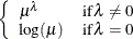
POWERMINUS2
Power with exponent -2

RECIPROCAL
INVERSE
Reciprocal

The default link functions for the various distributions are shown in Table 51.5.
- NOINT
-
requests that no intercept be included in the model. An intercept is included by default, unless the distribution is DIST= CONSTANT or DIST= UNIFORM.
- OFFSET=variable
-
specifies the offset variable function for the linear predictor in the model. An offset variable can be thought of as a regressor variable whose regression coefficient is known to be 1. For example, you can use an offset in a Poisson model when counts have been obtained in time intervals of different lengths. With a log link function, you can model the counts as Poisson variables with the logarithm of the time interval as the offset variable.
-
PARAMETERS(parameter-specification)
PARMS(parameter-specification) -
specifies starting values for the model parameters. If no PARMS option is given, the HPFMM procedure determines starting values by a data-dependent algorithm. To determine initial values for the Markov chain with Bayes estimation, see also the INITIAL= option in the BAYES statement. The specification of the parameters takes the following form: parameters in the mean function precede the scale parameters, and parameters for different components are separated by commas.
The following statements specify starting parameters for a two-component normal model. The initial values for the intercepts are 1 and –3; the initial values for the variances are 0.5 and 4.
proc hpfmm;
   model y = / k=2 parms(1 0.5, -3 4);
run;
You can specify missing values for parameters whose starting values are to be determined by the default method. Only values for parameters that participate in the optimization are specified. The values for model effects are specified on the linear (linked) scale.