The GLIMMIX Procedure
-
Overview

-
Getting Started
-
SyntaxPROC GLIMMIX StatementBY StatementCLASS StatementCODE StatementCONTRAST StatementCOVTEST StatementEFFECT StatementESTIMATE StatementFREQ StatementID StatementLSMEANS StatementLSMESTIMATE StatementMODEL StatementNLOPTIONS StatementOUTPUT StatementPARMS StatementRANDOM StatementSLICE StatementSTORE StatementWEIGHT StatementProgramming StatementsUser-Defined Link or Variance Function
-
DetailsGeneralized Linear Models TheoryGeneralized Linear Mixed Models TheoryGLM Mode or GLMM ModeStatistical Inference for Covariance ParametersDegrees of Freedom MethodsEmpirical Covariance ("Sandwich") EstimatorsExploring and Comparing Covariance MatricesProcessing by SubjectsRadial Smoothing Based on Mixed ModelsOdds and Odds Ratio EstimationParameterization of Generalized Linear Mixed ModelsResponse-Level Ordering and ReferencingComparing the GLIMMIX and MIXED ProceduresSingly or Doubly Iterative FittingDefault Estimation TechniquesDefault OutputNotes on Output StatisticsODS Table NamesODS Graphics
-
ExamplesBinomial Counts in Randomized BlocksMating Experiment with Crossed Random EffectsSmoothing Disease Rates; Standardized Mortality RatiosQuasi-likelihood Estimation for Proportions with Unknown DistributionJoint Modeling of Binary and Count DataRadial Smoothing of Repeated Measures DataIsotonic Contrasts for Ordered AlternativesAdjusted Covariance Matrices of Fixed EffectsTesting Equality of Covariance and Correlation MatricesMultiple Trends Correspond to Multiple Extrema in Profile LikelihoodsMaximum Likelihood in Proportional Odds Model with Random EffectsFitting a Marginal (GEE-Type) ModelResponse Surface Comparisons with Multiplicity AdjustmentsGeneralized Poisson Mixed Model for Overdispersed Count DataComparing Multiple B-SplinesDiallel Experiment with Multimember Random EffectsLinear Inference Based on Summary DataWeighted Multilevel Model for Survey DataQuadrature Method for Multilevel Model
- References
Kenward-Roger Degrees of Freedom Approximation
The DDFM=
KENWARDROGER option prompts PROC GLIMMIX to compute the denominator degrees of freedom in t tests and F tests by using the approximation described in Kenward and Roger (1997). For inference on the linear combination  in a Gaussian linear model, they propose a scaled Wald statistic
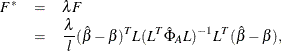
where  ,
,  is a bias-adjusted estimator of the precision of
  , and
, and  . An appropriate
  approximation to the sampling distribution of
  is derived by matching the first two moments of with those from the approximating F distribution and solving for the values of
  and m. The value of m thus derived is the Kenward-Roger degrees of freedom. The precision estimator is bias-adjusted, in contrast to the conventional precision estimator
  , which is obtained by simply replacing
  with
with  in
in  , the asymptotic variance of . This method uses to address the fact that
  is a biased estimator of , and itself underestimates
  when is unknown. This bias-adjusted precision estimator is also discussed in Prasad and Rao (1990); Harville and Jeske (1992); Kackar and Harville (1984).
By default, the observed information matrix of the covariance parameter estimates is used in the calculations.
For covariance structures that have nonzero second derivatives with respect to the covariance parameters, the Kenward-Roger
covariance matrix adjustment includes a second-order term. This term can result in standard error shrinkage. Also, the resulting
adjusted covariance matrix can then be indefinite and is not invariant under reparameterization. The FIRSTORDER suboption
of the DDFM=KENWARDROGER option eliminates the second derivatives from the calculation of the covariance matrix adjustment.
For scalar estimable functions, the resulting estimator is referred to as the Prasad-Rao estimator  in Harville and Jeske (1992). You can use the COVB(DETAILS)
option to diagnose the adjustments that PROC GLIMMIX makes to the covariance matrix of fixed-effects parameter estimates.
An application with DDFM=KENWARDROGER is presented in Example 45.8. The following are examples of covariance structures that generally lead to nonzero second derivatives: TYPE=ANTE(1)
, TYPE=AR(1)
, TYPE=ARH(1)
, TYPE=ARMA(1,1)
, TYPE=CHOL
, TYPE=CSH
, TYPE=FA0(q)
, TYPE=TOEPH
, TYPE=UNR
, and all TYPE=SP()
structures.
in Harville and Jeske (1992). You can use the COVB(DETAILS)
option to diagnose the adjustments that PROC GLIMMIX makes to the covariance matrix of fixed-effects parameter estimates.
An application with DDFM=KENWARDROGER is presented in Example 45.8. The following are examples of covariance structures that generally lead to nonzero second derivatives: TYPE=ANTE(1)
, TYPE=AR(1)
, TYPE=ARH(1)
, TYPE=ARMA(1,1)
, TYPE=CHOL
, TYPE=CSH
, TYPE=FA0(q)
, TYPE=TOEPH
, TYPE=UNR
, and all TYPE=SP()
structures.
DDFM=
KENWARDROGER2 specifies an improved F approximation of the DDFM=
KENWARD-ROGER type that uses a less biased precision estimator, as proposed by Kenward and Roger (2009). An important feature of the KR2 precision estimator is that it is invariant under reparameterization within the classes
of intrinsically linear and intrinsically linear inverse covariance structures. For the invariance to hold within these two
classes of covariance structures, a modified expected Hessian matrix is used in the computation of the covariance matrix of
. The two cells classified as "Modified" scoring for RxPL estimation in Table 45.23 give the modified Hessian expressions for the cases where the scale parameter is profiled and not profiled. You can enforce
the use of the modified expected Hessian matrix by specifying both the EXPHESSIAN and SCOREMOD options in the PROC GLIMMIX
statement. Kenward and Roger (2009) note that for an intrinsically linear covariance parameterization, DDFM=
KR2 produces the same precision estimator as that obtained using DDFM=
KR(FIRSTORDER).