Shared Concepts and Topics

Myers (1976) analyzes an experiment reported by Frankel (1961) that is aimed at maximizing the yield of mercaptobenzothiazole (MBT) by varying processing time and temperature. Myers uses a two-factor model in which the estimated surface does not have a unique optimum. The objective is to find the settings of time and temperature in the processing of the chemical that maximize the yield. The following statements create the data set d:

data d;
   input Time Temp MBT @@;
   label Time = "Reaction Time (Hours)"
         Temp = "Temperature (Degrees Centigrade)"
         MBT  = "Percent Yield Mercaptobenzothiazole";
   datalines;
 4.0  250  83.8    20.0  250  81.7    12.0  250  82.4
12.0  250  82.9    12.0  220  84.7    12.0  280  57.9
12.0  250  81.2     6.3  229  81.3     6.3  271  83.1
17.7  229  85.3    17.7  271  72.7     4.0  250  82.0
;

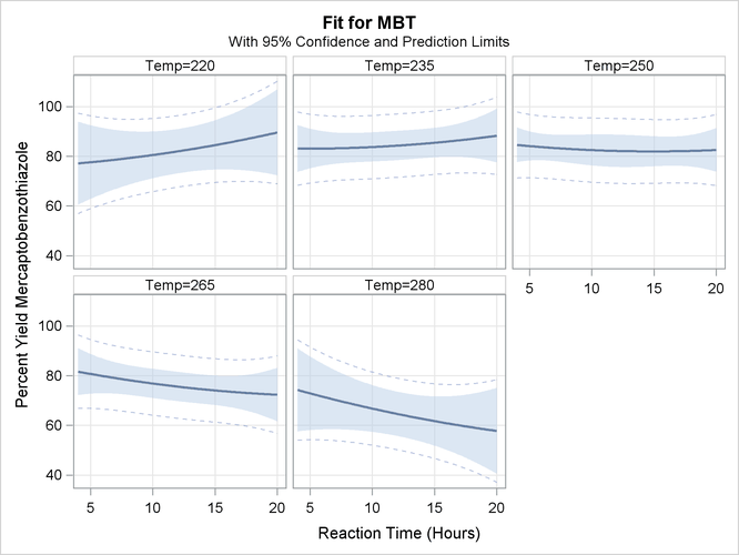
In the following statements, the ORTHOREG procedure fits a response surface regression model to the data and uses the EFFECTPLOT statement to create a slice of the response surface. The FIT plot-type requests plots of the predicted yield against the Time variable, and the PLOTBY= option specifies that the Temp variable is fixed at five equally spaced values so that five fitted regression curves are displayed in Output 19.1.1.

ods graphics on;
proc orthoreg data=d;
   model MBT=Time|Time|Temp|Temp@2;
   effectplot fit(x=time plotby=temp);
run;
ods graphics off;

The displays in Output 19.1.1 show that the slope of the surface changes as the temperature increases.

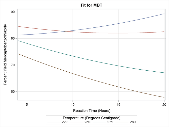
It might be more informative to see these results in one graphic, so the following statements specify the SLICEFIT plot-type to overlay plots of the predicted yield versus time, fixed at several values of temperature. In this case, the SLICEBY= option is specified to explicitly use the same four temperatures as used in the experiment.

ods graphics on;
proc orthoreg data=d;
   model MBT=Time|Time|Temp|Temp@2;
   effectplot slicefit(x=time sliceby=temp=229 250 271 280);
run;
ods graphics off;

Output 19.1.2 shows that to optimize the yield you should choose either low temperatures and long times or high temperatures and short times.

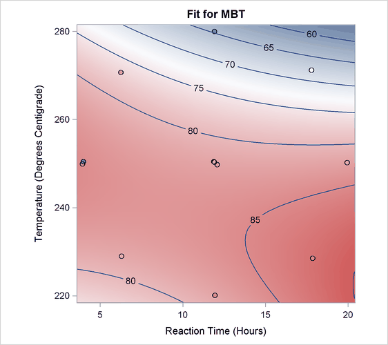
Another plot might explain the reason for these conflicting results more clearly. The following statements produce the default EFFECTPLOT statement display, enhanced by the OBS(JITTER) option to jitter the observations so that you can see the replicated points:

ods graphics on;
proc orthoreg data=d;
   model MBT=Time|Time|Temp|Temp@2;
   effectplot / obs(jitter(seed=39393));
run;
ods graphics off;

Output 19.1.3 shows that the reason for the changing slopes is that the surface is at a saddle point. This surface does not have an optimum point.