You can specify the following EFFECTPLOT options.
- ADDCELL<=value>
-
adds value to the weight of every cell in the MOSAIC plot-type. You can specify value as any nonnegative number. If you do not specify a value, then value=0.5. This enables you to add some dimension to zero frequency cells.
- ALPHA=value
-
specifies the significance level,
 value
value  , for producing
  prediction and confidence limits. By default, value=0.05.
-
AT <contopt> <classopt> <variable1<(CODED)>=varopt <variable2<(CODED)>=varopt…>>
where contopt= MEAN | MIN | MAX | MIDRANGE
classopt= ALL | REF
varopt= contopts | number-list | classopts | ’class-level’…’class-level’ -
specifies values at which to fix continuous and CLASS variables when they are not used in X=, Y=, SLICEBY=, or PLOTBY= effects. The contopt keyword fixes continuous variables at their mean, minimum, maximum, or midrange
 ; the default is to use the mean. The classopt keyword either fixes a CLASS variable at its reference (last) level or indicates that all levels of the CLASS variable should
be processed; the default is to use the reference level. The varopt values enable you to specify contopt and classopt keywords or to specify lists of numbers or class levels. You can specify a CLASS variable only once in the AT specification,
but you can specify a continuous variable multiple times; for example, the following syntax is valid when
; the default is to use the mean. The classopt keyword either fixes a CLASS variable at its reference (last) level or indicates that all levels of the CLASS variable should
be processed; the default is to use the reference level. The varopt values enable you to specify contopt and classopt keywords or to specify lists of numbers or class levels. You can specify a CLASS variable only once in the AT specification,
but you can specify a continuous variable multiple times; for example, the following syntax is valid when Xis a continuous variable:effectplot / at(x=min max x=0 to 2 by 1 x=2 5 7);
Duplicate AT values are suppressed, so the last
X=2 value is ignored.You can also specify coded plug-in values for CLASS variable levels when computing the predicted values
 . For example, suppose a CLASS variable
 Awith two levels={0,1} is in the model. Then instead of using the coding forAin the vector by specifying
 AT(A=all),AT(A=ref)orAT(A=’0’ ’1’), you can specify a numeric list to plug in. For example, if the proportion of A’s that equal 0 in the data set is 0.3, then you can input the proportions for all levels of the variable by specifyingAT(A(CODED)=0.3 0.7). Under GLM coding,A=0 is coded as “1 0” andA=1 is coded as “0 1”, so the plug-in specification replaces both of these codings with “0.3 0.7”. Under REFERENCE coding,A=0 is coded as “1” andA=1 is coded as “0”, so this specification replaces both of these codings with “0.3” followed by “0.7”; however, if another variable is nested withinA, then only “0.3” is used. To plug in values, you must specify a multiple of the number of parameters used for the CLASS variable or, if a variable is nested within the CLASS variable, a multiple of the number of levels of the CLASS variable.The coded plug-in values are distributed through the rest of the model effects in the following fashion. If a variable is nested within a plug-in variable, then its coding is multiplied by the plug-in value for the level it is nested in. If a variable interacts with a plug-in variable, its coding is multiplied by the appropriate plug-in value for the level it is interacting with. Lag, multimember, polynomial, and spline constructed effects are affected only by interactions and nestings. If the plug-in variable is part of a collection effect, then its values are replaced by the plug-in values; collection effects are also affected by interactions and nestings.
The AT levels are used for computing the predicted values. If the OBS option is also specified, then all observations are still displayed in all the plots. For example, if you specify the options
AT(A=’1’) OBS, then the fitted values are computed by usingA=1, but all the observations are displayed with their predicted values computed at their observed level ofA. If you want to display only a subset of the observations based on the levels of a CLASS variable, then you must specify either the PLOTBY= option or the OBS(BYAT) option. - ATLEN=n
-
specifies the maximum length (1
 n 256) of the levels of
the AT variables that are displayed in footnotes and headers. By default, up to 256 characters of the CLASS levels are displayed,
and the continuous AT levels are displayed with a BEST format that has a width greater than or equal to 5, which distinguishes
each level.
Caution: If the levels of your AT variables are not unique when the first n characters are displayed, then the levels are combined in the plots but not in the underlying computations. Also, at most
n characters for continuous AT variables are displayed.
n 256) of the levels of
the AT variables that are displayed in footnotes and headers. By default, up to 256 characters of the CLASS levels are displayed,
and the continuous AT levels are displayed with a BEST format that has a width greater than or equal to 5, which distinguishes
each level.
Caution: If the levels of your AT variables are not unique when the first n characters are displayed, then the levels are combined in the plots but not in the underlying computations. Also, at most
n characters for continuous AT variables are displayed.
- ATORDER=ASCENDING | DESCENDING
-
uses the AT values for continuous variables in ascending or descending order as specified. By default, values are used in the order of their first appearance in the AT option.
- BIN
-
displays the statistic for the MOSAIC plot-type with a discrete coloring scheme.
- CLI
-
displays normal (Wald) prediction limits. This option is available only for normal distributions with identity links. If your model is from a Bayesian analysis, then sampling-based intervals are computed; for more information, see the section Analysis Based on Posterior Estimates in Chapter 73: The PLM Procedure.
- CLM
-
displays confidence limits. These are computed as the normal (Wald) confidence limits for the linear predictor, and if the ILINK option is specified, the limits are also back-transformed by the inverse link function. If your model is from a Bayesian analysis, then sampling-based intervals are computed; for more information, see the section Analysis Based on Posterior Estimates in Chapter 73: The PLM Procedure.
- CLUSTER<=percent>
-
modifies the BOX and INTERACTION plot-types by displaying the levels of the SLICEBY= effect side by side. You can specify percent as a percentage of half the distance between X levels. The percent value must be between 0.1 and 1; the default percent depends on the number of X levels, the number of SLICEBY levels, and the number of PLOTBY levels for INTERACTION plot-types. You can remove default clustering by specifying the NOCLUSTER option.
- CONNECT
-
modifies the BOX and INTERACTION plot-types by connecting the predicted values with a line. You can remove default connecting lines by specifying the NOCONNECT option.
- EQUAL
-
causes every cell in the MOSAIC plot-type to have the same dimensions.
- EXTEND=DATA | value
-
extends continuous covariate axes by
 in both directions, where
  is the range of the X axis. Specifying the DATA keyword displays curves to the range of the data within the appropriate SLICEBY=, PLOTBY=, and AT level. For the CONTOUR plot-type, value=0.05 by default; other plot-types set the default value to 0. When constructed effects are present, only the EXTEND=DATA option is available.
- GRIDSIZE=n
-
specifies the resolution of curves by computing the predicted values at n equally spaced values on the X axis and specifies the resolution of surfaces by computing the predicted values on an n
 n grid of points. Default values are n = 200 for curves and bands, n = 50 for surfaces, and n = 2 for lines. If results of a Bayesian or bootstrap analysis are being displayed, then the defaults are n = 500000/B, where B is the number of samples, the upper limit is equal to the usual defaults, and the lower limit is equal to 20.
- ILINK
-
displays the fit on the scale of the inverse link function. In particular, the results are displayed on the probability scale for logistic regression. By default, a procedure displays the fit on either the link or inverse link scale.
- INDIVIDUAL
-
displays individual probabilities for polytomous response models with cumulative links on the scale of the inverse link function. This option is not available when the LINK option is specified, and confidence limits are not available when you specify this option.
- LIMITS
- LINK
-
displays the fit on the scale of the link function—that is, the linear predictor. Probabilities or observed proportions near 0 and 1 are transformed to
 . By default, a procedure displays the fit on either the link or inverse link scale.
- MOFF
-
moves the offset for a Poisson regression model to the response side of the equation. If the ILINK option is also specified, then the rate is displayed on the Y axis; if the LINK option is also specified, then the log of the rate is displayed on the Y axis. Without the MOFF option, the predicted values are computed and displayed only for the observations.
- NCOLS=n
-
specifies the maximum number of columns in a paneled plot. This option is not available with the BOX plot-type.
The default choice of NROWS= and NCOLS= is based on the number of PLOTBY= and AT levels. If only one plot is displayed in a panel, then NROWS=1 and NCOLS=1 and the plots are produced as if you specified only the UNPACK option. If only two plots are displayed in a panel, then NROWS=1 and NCOLS=2. For all other cases, a 2
2, 23, or 33 panel is chosen based on how much of the last panel is used, with ties going to the larger panels. For example, if 14 plots
are being created, then this requires either four 22 panels with 50% of the last panel filled, three 23 panels with 33% of the last panel filled, or two 33 panels with 55% of the last panel filled; in this case, the 33 panels are chosen.
If you specify both the NROWS= and NCOLS= options, then those are the values used. However, if you specify only one of the options but have fewer plots, then the panel size is reduced; for example, if you specify NROWS=6 but have only four plots, then a plot that has four rows and one column is produced.
- NOBORDER
-
removes the border from the cells in the MOSAIC plot-type. Otherwise, the color of the cells that were not observed in the data set is hidden by the border.
- NOCLI
- NOCLM
- NOCLUSTER
-
modifies the BOX and INTERACTION plot-types by preventing the side-by-side display of the levels of the SLICEBY= effect.
- NOCONNECT
-
modifies the BOX and INTERACTION plot-types by suppressing the line that connects the predicted values.
- NOLIMITS
- NOOBS
-
suppresses the display of observations and overrides the specification of the OBS= option.
- NROWS=n
-
specifies the maximum number of rows in a paneled plot. This option is not available with the BOX plot-type. For more information, see the NCOLS= option.
- OBS<(obs-options)>
-
displays observations in the effect plots. An input data set is required; hence the OBS option is not available with PROC PLM. The OBS option is overridden by the NOOBS option. When the ILINK option is specified with binary response variables, then either the observed proportions or a coded value of the response is displayed. For polytomous response variables, the observed values are overlaid onto the fitted curves unless the LOCATION= option is specified. Whether or not observations are displayed by default depends on the procedure. If the PLOTBY= option is specified, then the observations that are displayed in each plot are from the corresponding PLOTBY= level for classification effects; for continuous effects, all observations are displayed in every plot.
You can specify the following obs-options:
- BYAT
-
subsets the observations by AT level and by the PLOTBY= level. If you specify the PLOTBY= option without specifying this option, the observations are displayed in the plots that correspond to their PLOTBY= level without regard to any classification variables specified in the AT option. However, for FIT plot-types a distance can be computed and displayed (for more information, see the DISTANCE option). This option is ignored when there are no AT variables.
- CDISPLAY=NONE | OUTLINE | GRADIENT | OUTLINEGRADIENT
-
controls the display of observations in contour plots. The keyword OUTLINE displays the observations as circles, GRADIENT displays gradient-colored dots, OUTLINEGRADIENT displays gradient-filled-circles, and NONE suppresses the display of the observations. The default is CDISPLAY=OUTLINEGRADIENT.
- CGRADIENT=RESIDUAL | DEPENDENT
-
specifies what the gradient shading of the observed values in the CONTOUR plot-type represents. The RESIDUAL keyword shades the observations by the raw residual value and displays the fitted surface as a line contour plot. The DEPENDENT keyword shades the observations by the response variable value and displays the fitted surface as a contour shaded on the same scale. The default is CGRADIENT=DEPENDENT.
- DEPTH=depth
-
specifies the number of overlapping observations that can be distinguished by adjusting their transparency; you can specify 1
depth 100. By default, DEPTH=1. The DEPTH= option is available with the FIT, SLICEFIT, and INTERACTION plot-types.
- DISTANCE
-
displays observations in FIT plot-types with a color gradient that indicates how far the observation is from the AT and PLOTBY= level. This option is ignored unless an AT or PLOTBY= option is specified.
The distance is computed as the square root of the following number: for each continuous AT and PLOTBY= variable, add the square of the difference from the observed value divided by the range of the variable; for each CLASS AT and PLOTBY= variable, add 1 if the CLASS levels are different. Thus the largest possible distance is the square root of the number of AT and PLOTBY= variables. Observations at zero distance are displayed by using the darkest color, and the color fades as the distance increases.
The unpacked panels compute the maximum distance within each panel and hence do not use the same gradient across all panels. Also, the PANELS panel-type computes the maximum distance within each PLOTBY= level, so a different gradient is used for each PLOTBY= level. All other panel-types compute the maximum distance across all observations and therefore use the same gradient in every plot.
- FITATCLASS
-
computes fitted values only for class levels that are observed in the data set. This option is ignored when the GLM parameterization is used.
- FRINGE
-
displays observations in a fringe (rug) plot at the bottom of the plot. This option is available only with the FIT and SLICEFIT plot-types.
- JITTER<(jitter-options)>
-
shifts (jitters) the observations. By default, the jittering in the X direction is achieved by adding a random number that is generated according to a normal distribution with mean=0 and standard deviation
 and truncating at
  , where x-jitter=0.01 times the range of the X axis; the jittering in the Y direction is performed independently but in the same fashion.
The JITTER option is not available with the BOX plot-type. You can specify the following jitter-options:
, where x-jitter=0.01 times the range of the X axis; the jittering in the Y direction is performed independently but in the same fashion.
The JITTER option is not available with the BOX plot-type. You can specify the following jitter-options:
- FACTOR=factor
-
sets the jitter to factor times the range of the axis, and jitters in both the X and Y directions. You can specify
 .
.
- SEED=seed
-
specifies an integer to use as the initial seed for the random number generator. If you do not specify a seed, or if you specify a value less than or equal to zero, then the time of day from the computer clock is used to generate an initial seed.
- X=x-jitter
-
sets the jitter to x-jitter for the X direction; the jitter in the Y direction is assumed to be 0 unless the Y= option is also specified. You can specify
 . The X= option is not available for the INTERACTION plot-type. This option is ignored if the FACTOR= option is also specified.
- Y=y-jitter
-
sets the jitter to y-jitter for the Y direction; the jitter in the X direction is assumed to be 0 unless the X= option is also specified. You can specify
 . This option is ignored if the FACTOR= option is also specified.
- LABEL<=OBS>
-
labels markers with their observation number.
- LOCATION=location
-
specifies where the observed values for polytomous response models are displayed when the SLICEBY= variable is the response. This option is available only with the SLICEFIT and INTERACTION plot-types. The observations are always displayed at their appropriate X-axis value, but their Y-axis location can depend on the specification of the YRANGE= option or on the minimum and maximum computed predicted values in addition to the specified location. You can specify the following locations:
- BOTTOM<=factor>
-
displays the first response level at the minimum predicted value, and displays succeeding response levels above the first level at
 intervals, where is the range of the predicted values. You can specify
  , but the largest usable value, which corresponds to LOCATION=SPREAD, is factor=
 , where
  is the number of response levels that are displayed. By default, factor=0.03.
- CURVE
-
displays the observations for polytomous response models at their predicted values. For displays on the LINK scale, the reference level is displayed at the maximum value. This method is the default.
- FIRST
-
displays the observations for a response level at the first displayed predicted value for that response level.
- MAX
-
displays the observations for a response level at the maximum displayed predicted value for that response level.
- MIDDLE
-
displays the observations for a response level at the middle of the displayed predicted values for that response level.
- MIN
-
displays the observations for a response level at the minimum displayed predicted value for that response level.
- SPREAD
-
displays the observations with the response levels evenly spread across the Y axis.
- TOP<=factor>
-
displays the last response level at the maximum predicted value, and displays preceding response levels below the last level at
intervals, where is the range of the predicted values. You can specify , but the largest usable value, which corresponds to LOCATION=SPREAD, is factor=, where k+1 is the number of response levels that are displayed. By default, factor=0.03.
- PLOTBY<(panel-type)>=effect<=numeric-list>
-
specifies a variable or CLASS effect at whose levels the predicted values are computed and the plots are displayed. You can specify the response variable as the effect for polytomous response models. The panel-type argument specifies the method in which the plots are grouped for the display. You can specify the following panel-types:
This option is ignored with the BOX plot-type; box plots are always displayed in an unpacked fashion, grouped by the PLOTBY= and AT levels. If you specify a continuous variable as the effect, then either you can specify a numeric-list of values at which to display that variable or, by default, five equally spaced values from the minimum variable value to its maximum are displayed.
The default panel-type is based on the number of PLOTBY= and AT levels, as shown in the following table.
Number of
PLOTBY= LevelsNumber of
AT LevelsResulting
panel-type1
1
(UNPACK)
>1
1
PACK
1
>1
PACK
2
>1
ROWS
3
>1
COLUMNS
>3
>1
PANELS
The default dimensions of the panels are also based on the number of PLOTBY= and AT levels; for more information, see the NCOLS= option.
Specification of the panel-type is honored except in the following cases. If you specify a panel-type but produce only one plot, specify the NROWS=1 and NCOLS=1 options, or specify the UNPACK option, then the plots are produced as if you specified only the UNPACK option. If you specify the PANELS panel-type with only one AT level, then the plots are produced with the UNPACK option. However, if you specify the PANELS panel-type but the PLOTBY= effect has only one level, then the panel-type is changed to PACK.
- PLOTBYLEN=n
-
specifies the maximum length (
 ) of the levels of
the PLOTBY= variables, which are displayed in footnotes and headers. By default, up to 256 characters of the CLASS levels are displayed.
Caution: If the levels of your PLOTBY= variables are not unique when the first n characters are displayed, then the levels are combined in the plots but not in the underlying computations.
) of the levels of
the PLOTBY= variables, which are displayed in footnotes and headers. By default, up to 256 characters of the CLASS levels are displayed.
Caution: If the levels of your PLOTBY= variables are not unique when the first n characters are displayed, then the levels are combined in the plots but not in the underlying computations.
- POLYBAR
-
displays polytomous response data as a stacked histogram whose bar heights are defined by the individual predicted value. Your response variable must be the effect that is specified in the SLICEBY= option. If you specify the INDIVIDUAL option, then the histogram bars are displayed side by side. If you specify the CLM option, then error bars are displayed on the side-by-side histogram bars.
- PREDLABEL='label'
-
specifies a label to be displayed on the Y axis. The default Y-axis label is determined by your model. For the CONTOUR plot-type, this option changes the title to “label for Y.”
- SHOWCLEGEND
-
displays the gradient legend for the CONTOUR plot-type. This option has no effect when the OBS(CGRADIENT=RESIDUAL) option is also specified.
- SLICEBY=NONE | effect<=numeric-list>
-
displays the fitted values at the different levels of the specified variable or CLASS effect. You can specify the response variable as the effect for polytomous response models. Use this option to modify the SLICEFIT, INTERACTION, and BOX plot-types. If you specify a continuous variable as the effect, then either you can specify a numeric-list of values at which to display that variable or, by default, five equally spaced values from the minimum variable value to its maximum are displayed. The NONE keyword is available for preventing the INTERACTION plot-type from slicing by a second classification covariate. The SLICEBY=NONE option is not available for the SLICEFIT plot-type, because that is the same as the FIT plot-type. The BOX plot-type accepts only classification effects.
- SMOOTH
-
overlays a loess smooth on the FIT plot-type for models that have only one continuous predictor. This option is not available for binary or polytomous response models.
- TYPE=PREDICTED | PARQUET | GOF
-
specifies the type of display for the MOSAIC plot-types. For effects that are specified as in the X= option, the TYPE=PREDICTED and TYPE=GOF mosaic plots create cells by dividing the X axis proportional to the total weight in each level of the x-effect, then dividing the Y axis according to the weight in each level of the y-effect within the x-effect levels, and dividing the X2 axis according to the weight in each level of the x2-effect within the x-effect and y-effect levels. The TYPE=PARQUET plot uses the predicted probabilities instead of the weights to determine the dimensions of the cells.
The default TYPE=PREDICTED mosaic plot colors the cells according to their predicted values (probabilities for binary and polytomous response models) computed at the AT and PLOTBY levels. The TYPE=GOF plot displays the Pearson goodness-of-fit statistic as in Friendly (2000), with the expected value computed at the AT and PLOTBY levels. For a cell
 defined by the axis levels, the PLOTBY and AT levels, and the response level
  , let
, let  be the sum of all the weights of the observations in that cell, let
  be the sum of the weights across all response levels, and let
  be the predicted response for that cell, where is the event level for binary response models, and
 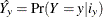 for binary and multinomial models. Then the Pearson goodness-of-fit statistic is computed as
![\[ \frac{W_{i_ y}-W_{i}\hat{Y}}{\sqrt {W_{i}\hat{Y}}} \]](images/statug_introcom0089.png)
The TYPE=GOF plot is not available when you have continuous covariates in the model. The TYPE=PARQUET plot shades the cells with their observed weights and is available only with binary or polytomous response data.
- UNPACK
-
suppresses paneling. By default, multiple plots can appear in some output panels. Specify UNPACK to display each plot separately.
- X=effect | (x-effect <y-effect <x2-effect>>)
-
specifies values to display on the X axis. For the BOX and INTERACTION plot-types, effect can be a CLASS effect in the MODEL statement. For the FIT, SLICEFIT, and CONTOUR plot-types, effect can be any continuous variable in the model. For the MOSAIC plot-types, you can specify CLASS effects (or the response variable if you have a multinomial model) as the effect or x-effect to display on the X axis, as the y-effect to display on the Y axis, and as the x2-effect to display on the X2 (upper) axis.
- Y=args
-
specifies values to display on the Y axis for the CONTOUR plot-type. The Y= argument can be any continuous variable in the model.
- YRANGE=CLIP | (<min><,max>)
-
displays the predicted values on the Y axis in the range [min,max]. The YRANGE=CLIP option has the same effect as specifying the minimum predicted value as min and the maximum predicted value as max. The axis might extend beyond your specified values. By default, when the Y axis displays predicted probabilities, the entire Y axis, [0,1], is displayed. This option is useful if your predicted probabilities are all contained in some subset of this range. This option is not available with the CONTOUR plot-type.