The GLMPOWER Procedure

The univariate linear model has the form
where ![]() is the
is the ![]() vector of responses,
vector of responses, ![]() is the
is the ![]() design matrix,
design matrix, ![]() is the
is the ![]() vector of model parameters corresponding to the columns of
vector of model parameters corresponding to the columns of ![]() , and
, and ![]() is an
is an ![]() vector of errors with
vector of errors with
In PROC GLMPOWER, the model parameters ![]() are not specified directly, but rather indirectly as
are not specified directly, but rather indirectly as ![]() , which represents either conjectured response means or typical response values for each design profile. The
, which represents either conjectured response means or typical response values for each design profile. The ![]() values are manifested as the dependent variable in the MODEL statement. The vector
values are manifested as the dependent variable in the MODEL statement. The vector ![]() is obtained from
is obtained from ![]() according to the least squares equation,
according to the least squares equation,
Note that, in general, there is not a one-to-one mapping between ![]() and
and ![]() . Many different scenarios for
. Many different scenarios for ![]() might lead to the same
might lead to the same ![]() . If you specify
. If you specify ![]() with the intention of representing cell means, keep in mind that PROC GLMPOWER allows scenarios that are not valid cell means according to the model that is specified in the MODEL statement. For example, if
with the intention of representing cell means, keep in mind that PROC GLMPOWER allows scenarios that are not valid cell means according to the model that is specified in the MODEL statement. For example, if ![]() exhibits an interaction effect but the corresponding interaction term is left out of the model, then the cell means (
exhibits an interaction effect but the corresponding interaction term is left out of the model, then the cell means (![]() ) that are derived from
) that are derived from ![]() differ from
differ from ![]() . In particular, the cell means that are derived in this way are the projection of
. In particular, the cell means that are derived in this way are the projection of ![]() onto the model space.
onto the model space.
It is convenient in power analysis to parameterize the design matrix ![]() in three parts,
in three parts, ![]() , defined as follows:
, defined as follows:
-
The
 essence design matrix
  is the collection of unique rows of
  . Its rows are sometimes referred to as “design profiles.” Here,
  is defined simply as the number of unique rows of .
-
The
 weight vector
  reveals the relative proportions of design profiles, and
  . Row i of is to be included in the design
  times for every
  times that row j is included. The weights are assumed to be standardized (that is, they sum up to 1).
-
The total sample size is N. This is the number of rows in
. If you gather  copies of the
  th row of , for
  , then you end up with .
The preceding quantities are derived from PROC GLMPOWER syntax as follows:
It is useful to express the crossproduct matrix ![]() in terms of these three parts,
in terms of these three parts,
because this expression factors out the portion (N) that depends on sample size and the portion (![]() ) that depends only on the design structure.
) that depends only on the design structure.
A general linear hypothesis for the univariate model has the form
where ![]() is an
is an ![]() contrast matrix with rank
contrast matrix with rank ![]() and
and ![]() is the null value (usually just a vector of zeros).
is the null value (usually just a vector of zeros).
Note that model effect tests are just contrasts that use special forms of ![]() . Thus, this scheme covers both effect tests (which are specified in the MODEL statement and the EFFECTS= option in the POWER statement) and custom contrasts (which are specified in the CONTRAST statement).
. Thus, this scheme covers both effect tests (which are specified in the MODEL statement and the EFFECTS= option in the POWER statement) and custom contrasts (which are specified in the CONTRAST statement).
The model degrees of freedom ![]() are equal to the rank of
are equal to the rank of ![]() , denoted
, denoted ![]() . The error degrees of freedom
. The error degrees of freedom ![]() are equal to
are equal to ![]() . The sample size
. The sample size ![]() must be at least
must be at least ![]() plus the number of covariates.
plus the number of covariates.
The test statistic is
where
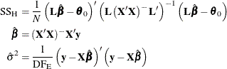
Under ![]() ,
, ![]() . Under
. Under ![]() , F is distributed as
, F is distributed as ![]() with noncentrality
with noncentrality
The value of ![]() is specified in the STDDEV= option in the POWER statement.
is specified in the STDDEV= option in the POWER statement.
Muller and Peterson (1984) give the exact power of the test as
The value of ![]() is specified in the ALPHA= option in the POWER statement.
is specified in the ALPHA= option in the POWER statement.
Sample size is computed by inverting the power equation.
See Muller and Benignus (1992) and O’Brien and Shieh (1992) for additional discussion.