Box-Cox Transformation Plot with PROC TRANSREG :: SAS/STAT(R) 12.3 User's Guide

Box-Cox Transformation Plot with PROC TRANSREG

This example is taken from Example 97.2 of Chapter 97: The TRANSREG Procedure. The following statements create a SAS data set that contains failure times for yarn:

proc format;
   value a -1 =   8 0 =   9 1 =  10;
   value l -1 = 250 0 = 300 1 = 350;
   value o -1 =  40 0 =  45 1 =  50;
run;

data yarn;
   input Fail Amplitude Length Load @@;
   format amplitude a. length l. load o.;
   label fail = 'Time in Cycles until Failure';
   datalines;
 674 -1 -1 -1    370 -1 -1  0    292 -1 -1  1    338  0 -1 -1
 266  0 -1  0    210  0 -1  1    170  1 -1 -1    118  1 -1  0

   ... more lines ...   

;

The following statements run PROC TRANSREG:

ods graphics on;

proc transreg data=yarn;
   model BoxCox(fail / convenient lambda=-2 to 2 by 0.05) =
         qpoint(length amplitude load);
run;

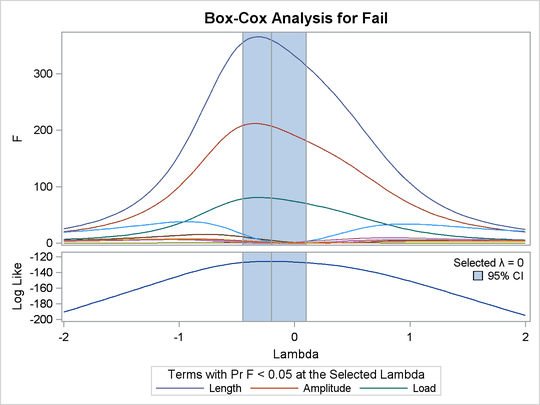
The log-likelihood plot in Figure 21.9 suggests a Box-Cox transformation with $\lambda = 0$ .

Figure 21.9: Box-Cox “Significant Effects”