H3: Congeneric (One-Factor) Model for Lord Data :: SAS/STAT(R) 12.3 User's Guide

H3: Congeneric (One-Factor) Model for Lord Data

The path diagram for this congeneric (one-factor) model is shown in Figure 17.20.

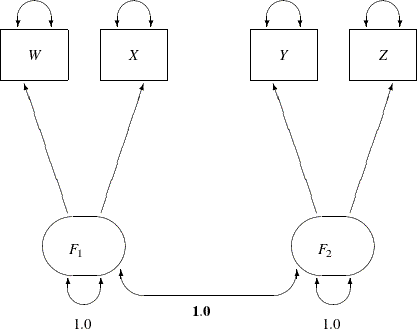
Figure 17.20: H3: Congeneric (One-Factor) Model for Lord Data

The only difference between the current path diagram in Figure 17.20 for the congeneric (one-factor) model and the preceding path diagram in Figure 17.17 for the full (two-factor) model is that the double-headed path that connects F1 and F2 is fixed to 1 in the current path diagram. Accordingly, you need to modify only slightly the preceding PROC CALIS specification to form the new model specification, as shown in the following statements:

proc calis data=lord;
   path   
      W <=== F1, 
      X <=== F1, 
      Y <=== F2,  
      Z <=== F2; 
   pvar 
      F1 = 1.0, 
      F2 = 1.0,
      W X Y Z;
   pcov
      F1 F2 = 1.0; 
run;

This specification sets the covariance between F1 and F2 to 1.0 in the PCOV statement. An annotated fit summary is displayed in Figure 17.21.

Figure 17.21: Fit Summary, H3: Congeneric (One-Factor) Model for Lord Data

Fit Summary
Chi-Square	36.2095
Chi-Square DF	2
Pr > Chi-Square	<.0001
Standardized RMR (SRMR)	0.0277
Adjusted GFI (AGFI)	0.8570
RMSEA Estimate	0.1625
Bentler Comparative Fit Index	0.9766

The chi-square value is 36.2095 (df = 2, p < 0.0001). This indicates that you can reject the hypothesized model at the 0.01 $\alpha$ -level. The standardized root mean square error (SRMSR) is 0.0277, which indicates a good fit. Bentler’s comparative fit index is 0.9766, which is also a good model fit. However, the adjusted GFI (AGFI) is 0.8570, which is not very impressive. Also, the RMSEA value is 0.1625, which is too large to be an acceptable model. Therefore, the congeneric model might not be the one you want to use.

The estimation results are displayed in Figure 17.22. Because the model does not fit well, the corresponding estimation results are not interpreted.

Figure 17.22: Estimation Results, H3: Congeneric (One-Factor) Model for Lord Data

PATH List
Path			Parameter	Estimate	Standard Error	t Value
W	<===	F1	_Parm1	7.10470	0.32177	22.08012
X	<===	F1	_Parm2	7.26908	0.31826	22.83973
Y	<===	F2	_Parm3	8.37344	0.32542	25.73143
Z	<===	F2	_Parm4	8.51060	0.32409	26.26002

Variance Parameters
Variance Type	Variable	Parameter	Estimate	Standard Error	t Value
Exogenous	F1		1.00000
	F2		1.00000
Error	W	_Parm5	35.92111	2.41467	14.87619
	X	_Parm6	33.42373	2.31037	14.46684
	Y	_Parm7	27.17043	2.24621	12.09613
	Z	_Parm8	25.38887	2.20837	11.49664

Covariances Among Exogenous Variables
Var1	Var2	Estimate	Standard Error	t Value
F1	F2	1.00000

Perhaps a more natural way to specify the model under hypothesis $H_{3}$ is to use only one factor in the PATH model, as shown in the following statements:

proc calis data=lord;
   path   
      W <=== F1, 
      X <=== F1, 
      Y <=== F1,  
      Z <=== F1; 
   pvar 
      F1 = 1.0, 
      W X Y Z;
run;

This produces essentially the same results as the specification with two factors that have perfect correlation.