The KRIGE2D Procedure

Ordinary Kriging

Denote the SRF by . Following the notation in Cressie (1993), the following model for is assumed:

Here, is the fixed, unknown mean of the process, and is a zero mean SRF, which represents the variation around the mean.

In most practical applications, an additional assumption is required in order to estimate the covariance of the process. This assumption is second-order stationarity:

This requirement can be relaxed slightly when you are using the semivariogram instead of the covariance. In this case, second-order stationarity is required of the differences rather than :

By performing local kriging, the spatial processes represented by the previous equation for are more general than they appear. In local kriging, at an unsampled location , a separate model is fit using only data in a neighborhood of . This has the effect of fitting a separate mean at each point, and it is similar to the kriging with trend (KT) method discussed in Journel and Rossi (1989).

Given the measurements at known locations , you want to obtain a prediction of at an unsampled location . When the following three requirements are imposed on the predictor , the OK predictor is obtained:

1. is linear in

2. is unbiased

3. minimizes the mean square prediction error

Linearity requires the following form for :

Applying the unbiasedness condition to the preceding equation yields

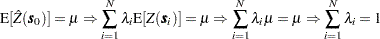Finally, the third condition requires a constrained linear optimization that involves and a Lagrange parameter . This constrained linear optimization can be expressed in terms of the function given by

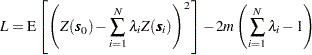Define the column vector by

and the column vector by

The optimization is performed by solving

in terms of and .

The resulting matrix equation can be expressed in terms of either the covariance or semivariogram . In terms of the covariance, the preceding equation results in the matrix equation

where

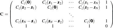and

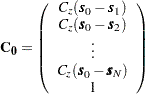The solution to the previous matrix equation is

Using this solution for and , the ordinary kriging prediction at is

with associated prediction error the square root of the variance

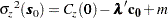where is with the in the last row removed, making it an vector.

These formulas are used in the best linear unbiased prediction (BLUP) of random variables (Robinson 1991). Further details are provided in Cressie (1993, pp. 119–123).

Because of possible numeric problems when solving the previous matrix equation, Deutsch and Journel (1992) suggest replacing the last row and column of s in the preceding matrix by , keeping the in the position and similarly replacing the last element in the preceding right-hand vector with . This results in an equivalent system but avoids numeric problems when is large or small relative to .