| Important Linear Algebra Concepts |
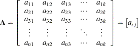
A matrix  is a rectangular array of numbers. The order of a matrix with
  rows and
  columns is
  . The element in row
  , column
  of is denoted as
  , and the notation
  is sometimes used to refer to the two-dimensional row-column array
 |
A vector is a one-dimensional array of numbers. A column vector has a single column ( ). A row vector has a single row (
 ). A scalar is a matrix of order
  —that is, a single number. A square matrix has the same row and column order,
  . A diagonal matrix is a square matrix where all off-diagonal elements are zero,
  if
if  . The identity matrix
  is a diagonal matrix with
  for all . The unit vector
  is a vector where all elements are
  . The unit matrix
  is a matrix of all s. Similarly, the elements of the null vector and the null matrix are all
  .
.
Basic matrix operations are as follows:
- Addition
-
If
and  are of the same order, then
  is the matrix of elementwise sums,
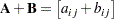
- Subtraction
-
If
and are of the same order, then  is the matrix of elementwise differences,
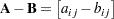
- Dot product
-
The dot product of two
-vectors  and
and  is the sum of their elementwise products,
The dot product is also known as the inner product of
and . Two vectors are said to be orthogonal if their dot product is zero. - Multiplication
-
Matrices
and are said to be conformable for  multiplication if the number of columns in equals the number of rows in
  . Suppose that is of order and that is of order
  . The product is then defined as the
  matrix of the dot products of the th row of and the th column of ,
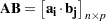
- Transposition
-
The transpose of the
matrix is denoted as  or
or  or
or  and is obtained by interchanging the rows and columns,
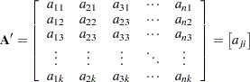
A symmetric matrix is equal to its transpose,
 . The inner product of two
  column vectors and is
  .
.
Matrix Inversion
Regular Inverses
The right inverse of a matrix is the matrix that yields the identity when is postmultiplied by it. Similarly, the left inverse of yields the identity if is premultiplied by it. is said to be invertible and is said to be the inverse of , if is its right and left inverse,  . This requires to be square and nonsingular. The inverse of a matrix is commonly denoted as
  . The following results are useful in manipulating inverse matrices (assuming both and
  are invertible):
 |
 |
|||
 |
 |
|||
 |
 |
|||
 |
 |
|||
 |
 |
If  is a diagonal matrix with nonzero entries on the diagonal—that is,
 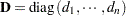 —then
—then 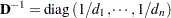 . If is a block-diagonal matrix whose blocks are invertible, then
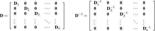 |
In statistical applications the following two results are particularly important, because they can significantly reduce the computational burden in working with inverse matrices.
- Partitioned Matrix
-
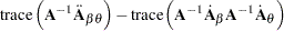
Suppose
is a nonsingular matrix that is partitioned as 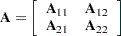
Then, provided that all the inverses exist, the inverse of
is given by 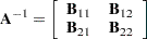
where
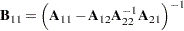 ,
, 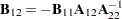 ,
, 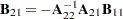 , and
, and 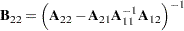 .
. - Patterned Sum
-
Suppose
 is
is  nonsingular,
  is
is  nonsingular, and and are and
  matrices, respectively. Then the inverse of
  is given by
This formula is particularly useful if
 and has a simple form that is easy to invert. This case arises, for example, in mixed models where might be a diagonal or block-diagonal matrix, and
  .
. Another situation where this formula plays a critical role is in the computation of regression diagnostics, such as in determining the effect of removing an observation from the analysis. Suppose that
 represents the crossproduct matrix in the linear model
  . If
. If  is the th row of the
  matrix, then
  is the crossproduct matrix in the same model with the th observation removed. Identifying
  ,
,  , and
, and  in the preceding inversion formula, you can obtain the expression for the inverse of the crossproduct matrix:
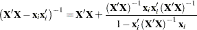
This expression for the inverse of the reduced data crossproduct matrix enables you to compute "leave-one-out" deletion diagnostics in linear models without refitting the model.
Generalized Inverse Matrices
If is rectangular (not square) or singular, then it is not invertible and the matrix does not exist. Suppose you want to find a solution to simultaneous linear equations of the form
 |
If is square and nonsingular, then the unique solution is  . In statistical applications, the case where is rectangular is less important than the case where is a square matrix of rank less than . For example, the normal equations in ordinary least squares (OLS) estimation in the model
  are
are
 |
A generalized inverse matrix is a matrix  such that
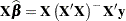
  is a solution to the linear system. In the OLS example, a solution can be found as
  , where
  is a generalized inverse of
  .
.
The following four conditions are often associated with generalized inverses. For the square or rectangular matrix there exist matrices that satisfy
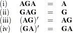 |
The matrix that satisfies all four conditions is unique and is called the Moore-Penrose inverse, after the first published work on generalized inverses by Moore (1920) and the subsequent definition by Penrose (1955). Only the first condition is required, however, to provide a solution to the linear system above.
Pringle and Rayner (1971) introduced a numbering system to distinguish between different types of generalized inverses. A matrix that satisfies only condition (i) is a  -inverse. The
  -inverse satistifes conditions (i) and (ii). It is also called a reflexive generalized inverse. Matrices satisfying conditions (i)–(iii) or conditions (i), (ii), and (iv) are
  -inverses. Note that a matrix that satisfies the first three conditions is a right generalized inverse, and a matrix that satisfies conditions (i), (ii), and (iv) is a left generalized inverse. For example, if is of rank , then
  is a left generalized inverse of . The notation
  -inverse for the Moore-Penrose inverse, satisfying conditions (i)–(iv), is often used by extension, but note that Pringle and Rayner (1971) do not use it; rather, they call such a matrix "the" generalized inverse.
If the matrix is rank-deficient—that is, 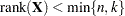 —then the system of equations
|
does not have a unique solution. A particular solution depends on the choice of the generalized inverse. However, some aspects of the statistical inference are invariant to the choice of the generalized inverse. If is a generalized inverse of , then  is invariant to the choice of . This result comes into play, for example, when you are computing predictions in an OLS model with a rank-deficient matrix, since it implies that the predicted values
 |
are invariant to the choice of  .
.
Matrix Differentiation
Taking the derivative of expressions involving matrices is a frequent task in statistical estimation. Objective functions that are to be minimized or maximized are usually written in terms of model matrices and/or vectors whose elements depend on the unknowns of the estimation problem. Suppose that and are real matrices whose elements depend on the scalar quantities  and
and  —that is,
  , and similarly for .
The following are useful results in finding the derivative of elements of a matrix and of functions involving a matrix. For more in-depth discussion of matrix differentiation and matrix calculus, see, for example, Magnus and Neudecker (1999) and Harville (1997).
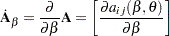
The derivative of with respect to is denoted  and is the matrix of the first derivatives of the elements of :
 |
Similarly, the second derivative of with respect to and is the matrix of the second derivatives
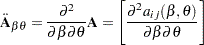 |
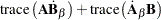
The following are some basic results involving sums, products, and traces of matrices:
 |
 |
|||
 |
 |
|||
 |
 |
|||
 |
 |
|||
 |
 |
|||
 |
 |
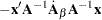
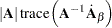
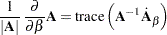
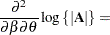
The next set of results is useful in finding the derivative of elements of and of functions of , if is a nonsingular matrix:
 |
 |
|||
 |
 |
|||
 |
 |
|||
 |
 |
|||
 |
 |
|||
 |
 |
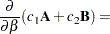
Now suppose that and are column vectors that depend on and/or and that  is a vector of constants. The following results are useful for manipulating derivatives of linear and quadratic forms:
 |
 |
|||
 |
 |
|||
 |
 |
|||
 |
 |
Matrix Decompositions
To decompose a matrix is to express it as a function—typically a product—of other matrices that have particular properties such as orthogonality, diagonality, triangularity. For example, the Cholesky decomposition of a symmetric positive definite matrix is  , where is a lower-triangular matrix. The spectral decomposition of a symmetric matrix is
  , where is a diagonal matrix and
  is an orthogonal matrix.
Matrix decomposition play an important role in statistical theory as well as in statistical computations. Calculations in terms of decompositions can have greater numerical stability. Decompositions are often necessary to extract information about matrices, such as matrix rank, eigenvalues, or eigenvectors. Decompositions are also used to form special transformations of matrices, such as to form a "square-root" matrix. This section briefly mentions several decompositions that are particularly prevalent and important.
LDU, LU, and Cholesky Decomposition
Every square matrix , whether it is positive definite or not, can be expressed in the form  , where
  is a unit lower-triangular matrix, is a diagonal matrix, and
  is a unit upper-triangular matrix. (The diagonal elements of a unit triangular matrix are 1.) Because of the arrangement of the matrices, the decomposition is called the LDU decomposition. Since you can absorb the diagonal matrix into the triangular matrices, the decomposition
 |
is also referred to as the LU decomposition of .
If the matrix is positive definite, then the diagonal elements of are positive and the LDU decomposition is unique. Furthermore, we can add more specificity to this result in that for a symmetric, positive definite matrix, there is a unique decomposition  , where is unit upper-triangular and is diagonal with positive elements. Absorbing the square root of into ,
  , the decomposition is known as the Cholesky decomposition of a positive-definite matrix:
 |
where is upper triangular.
If is symmetric nonnegative definite of rank , then we can extend the Cholesky decomposition as follows. Let  denote the lower-triangular matrix such that
 |
Then  .
.
Spectral Decomposition
Suppose that is an symmetric matrix. Then there exists an orthogonal matrix  and a diagonal matrix such that
  . Of particular importance is the case where the orthogonal matrix is also orthonormal—that is, its column vectors have unit norm. Denote this orthonormal matrix as . Then the corresponding diagonal matrix—
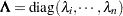 , say—contains the eigenvalues of . The spectral decomposition of can be written as
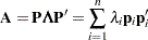 |
where  denotes the th column vector of . The right-side expression decomposes into a sum of rank-1 matrices, and the weight of each contribution is equal to the eigenvalue associated with the th eigenvector. The sum furthermore emphasizes that the rank of is equal to the number of nonzero eigenvalues.
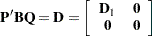
Harville (1997, p. 538) refers to the spectral decomposition of as the decomposition that takes the previous sum one step further and accumulates contributions associated with the distinct eigenvalues. If  are the distinct eigenvalues and
  , where the sum is taken over the set of columns for which
  , then
 |
You can employ the spectral decomposition of a nonnegative definite symmetric matrix to form a "square-root" matrix of . Suppose that  is the diagonal matrix containing the square roots of the
  . Then
  is a square-root matrix of in the sense that
  , because
 |
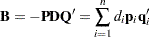
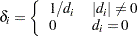
Generating the Moore-Penrose inverse of a matrix based on the spectral decomposition is also simple. Denote as  the diagonal matrix with typical element
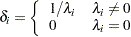 |
Then the matrix  is the Moore-Penrose (-generalized) inverse of .
Singular-Value Decomposition
The singular-value decomposition is related to the spectral decomposition of a matrix, but it is more general. The singular-value decomposition can be applied to any matrix. Let be an matrix of rank . Then there exist orthogonal matrices  and
and  of order and
  , respectively, and a diagonal matrix such that
 |
where  is a diagonal matrix of order . The diagonal elements of are strictly positive. As with the spectral decomposition, this result can be written as a decomposition of into a weighted sum of rank-1 matrices
 |
The scalars  are called the singular values of the matrix . They are the positive square roots of the nonzero eigenvalues of the matrix
  . If the singular-value decomposition is applied to a symmetric, nonnegative definite matrix , then the singular values
  are the nonzero eigenvalues of and the singular-value decomposition is the same as the spectral decomposition.
As with the spectral decomposition, you can use the results of the singular-value decomposition to generate the Moore-Penrose inverse of a matrix. If is with singular-value decomposition  , and if is a diagonal matrix with typical element
 |
then  is the -generalized inverse of .