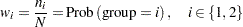
| The POWER Procedure |
Analyses in the TWOSAMPLEWILCOXON Statement
Wilcoxon-Mann-Whitney Test for Comparing Two Distributions (TEST=WMW)
The power approximation in this section is applicable to the Wilcoxon-Mann-Whitney (WMW) test as invoked with the WILCOXON option in the PROC NPAR1WAY statement of the NPAR1WAY procedure. The approximation is based on O’Brien and Castelloe (2006) and an estimator called  . See O’Brien and Castelloe (2006) for a definition of , which need not be derived in detail here for purposes of explaining the power formula.
Let  and
and  be independent observations from any two distributions that you want to compare using the WMW test. For purposes of deriving the asymptotic distribution of (and consequently the power computation as well), these distributions must be formulated as ordered categorical ("ordinal") distributions.
If a distribution is continuous, it can be discretized using a large number of categories with negligible loss of accuracy. Each nonordinal distribution is divided into  categories, where is the value of the NBINS parameter, with breakpoints evenly spaced on the probability scale. That is, each bin contains an equal probability
  / for that distribution. Then the breakpoints across both distributions are pooled to form a collection of
  bins (heretofore called "categories"), and the probabilities of bin membership for each distribution are recalculated. The motivation for this method of binning is to avoid degenerate representations of the distributions—that is, small handfuls of large probabilities among mostly empty bins—as can be caused by something like an evenly spaced grid across raw values rather than probabilities.
After the discretization process just mentioned, there are now two ordinal distributions, each with a set of probabilities across a common set of ordered categories. For simplicity of notation, assume (without loss of generality) the response values to be  . Represent the conditional probabilities as
 |
and the group allocation weights as
 |
The joint probabilities can then be calculated simply as
 |
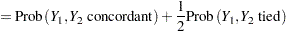
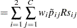
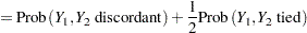
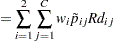
The next step in the power computation is to compute the probabilities that a randomly chosen pair of observations from the two groups is concordant, discordant, or tied. It is useful to define these probabilities as functions of the terms  and
and  , defined as follows, where
  is a random observation drawn from the joint distribution across groups and categories:
 |
 |
|||
 |
 |
|||
|
 |
|||
|
 |
and
 |
 |
|||
|
 |
|||
|
|
|||
|
 |
For an independent random draw  from the two distributions,
 |
 |
|||
|
 |
and
 |
 |
|||
|
 |
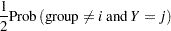
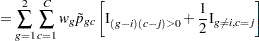
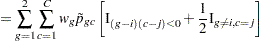
Then
 |
Proceeding to compute the theoretical standard error associated with  (that is, the population analogue to the sample standard error),
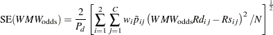 |
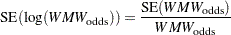
Converting to the natural log scale and using the delta method,
 |
The next step is to produce a "smoothed" version of the  cell probabilities that conforms to the null hypothesis of the Wilcoxon-Mann-Whitney test (in other words, independence in the contingency table of probabilities). Let
 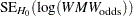 denote the theoretical standard error of
  assuming
  .
.
Finally we have all of the terms needed to compute the power, using the noncentral chi-square and normal distributions:
 |
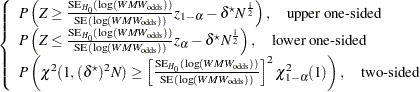 |
where
 |
is the primary noncentrality—that is, the "effect size" that quantifies how much the two conjectured distributions differ.  is a standard normal random variable,
  is a noncentral
  random variable with degrees of freedom
  and noncentrality
  , and
, and  is the total sample size.
Copyright © SAS Institute, Inc. All Rights Reserved.