| The MI Procedure |
| Discriminant Function Method for Monotone Missing Data |
The discriminant function method is the default imputation method for classification variables in a data set with a monotone missing pattern.
For a nominal classification variable  with responses 1, ...,
  and a set of effects from its preceding variables, if the covariates
  ,
,  , ...,
  associated with these effects within each group are approximately multivariate normal and the within-group covariance matrices are approximately equal, the discriminant function method (Brand 1999, pp. 95–96) can be used to impute missing values for the variable .
Denote the group-specific means for covariates , , ..., by
 |
then the pooled covariance matrix is computed as
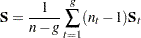 |
where  is the within-group covariance matrix,
  is the group-specific sample size, and
  is the total sample size.
In each imputation, new parameters of the group-specific means ( ), pooled covariance matrix (
 ), and prior probabilities of group membership (
 ) can be drawn from their corresponding posterior distributions (Schafer 1997, p. 356).
Pooled Covariance Matrix and Group-Specific Means
For each imputation, the MI procedure uses either the fixed observed pooled covariance matrix (PCOV=FIXED) or a drawn pooled covariance matrix (PCOV=POSTERIOR) from its posterior distribution with a noninformative prior. That is,
 |
 |
 |
where  is an inverted Wishart distribution.
The group-specific means are then drawn from their posterior distributions with a noninformative prior
 |
|
 |
See the section Bayesian Estimation of the Mean Vector and Covariance Matrix for a complete description of the inverted Wishart distribution and posterior distributions that use a noninformative prior.
Prior Probabilities of Group Membership
The prior probabilities are computed through the drawing of new group sample sizes. When the total sample size  is considered fixed, the group sample sizes
  have a multinomial distribution. New multinomial parameters (group sample sizes) can be drawn from their posterior distribution by using a Dirichlet prior with parameters
  .
.
After the new sample sizes are drawn from the posterior distribution of , the prior probabilities are computed proportionally to the drawn sample sizes.
See Schafer (1997, pp. 247–255) for a complete description of the Dirichlet prior.
Imputation Steps
The discriminant function method uses the following steps in each imputation to impute values for a nominal classification variable with responses:
Draw a pooled covariance matrix
from its posterior distribution if the PCOV=POSTERIOR option is used. For each group, draw group means
from the observed group mean  and either the observed pooled covariance matrix (PCOV=FIXED) or the drawn pooled covariance matrix (PCOV=POSTERIOR).
 For each group, compute or draw
, prior probabilities of group membership, based on the PRIOR= option: PRIOR=EQUAL,
 , prior probabilities of group membership are all equal.
 PRIOR=PROPORTIONAL,
 , prior probabilities are proportional to their group sample sizes.
 PRIOR=JEFFREYS=
 , a noninformative Dirichlet prior with
  is used.
 PRIOR=RIDGE=
 , a ridge prior is used with
  for
for  and
and  for
for  .
.
With the group means
, the pooled covariance matrix , and the prior probabilities of group membership , the discriminant function method derives linear discriminant function and computes the posterior probabilities of an observation belonging to each group 
where
 is the generalized squared distance from
  to group
  .
. Draw a random uniform variate
 , between 0 and 1, for each observation with missing group value. With the posterior probabilities,
  , the discriminant function method imputes
  if the value of is less than
  ,
,  if the value is greater than or equal to but less than
  , and so on.
Copyright © SAS Institute, Inc. All Rights Reserved.