| Introduction to Regression Procedures |
| Parameter Estimates and Associated Statistics |
The Least Squares Estimators
Least squares estimators of the regression parameters are found by solving the normal equations
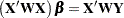 |
for the vector  , where
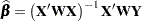
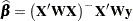
  is a diagonal matrix with the observed weights on the diagonal. The resulting estimator of the parameter vector is
 |
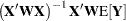
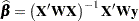
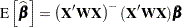
This is an unbiased estimator, since
 |
 |
|||
 |
 |
Notice that the only assumption necessary in order for the least squares estimators to be unbiased is that of a zero mean of the model errors. If the estimator is evaluated at the observed data, it is referred to Subidxleast squaresestimate (Introduction to Regression)as the least squares estimate,
 |
If the standard classical assumptions are met, the least squares estimators of the regression parameters are the best linear unbiased estimators (BLUE). In other words, the estimators have minimum variance in the class of estimators that are unbiased and that are linear functions of the responses. If the additional assumption of normally distributed errors is satisfied, then the following are true:
The statistics that are computed have the proper sampling distributions for hypothesis testing.
Parameter estimators are normally distributed.
Various sums of squares are distributed proportional to chi-square, at least under proper hypotheses.
Ratios of estimators to standard errors follow the Student’s
 distribution under certain hypotheses.
 Appropriate ratios of sums of squares follow an
 distribution for certain hypotheses.
When regression analysis is used to model data that do not meet the assumptions, the results should be interpreted in a cautious, exploratory fashion. The significance probabilities under these circumstances are unreliable.
Box (1966) and Mosteller and Tukey (1977, Chapters 12 and 13) discuss the problems that are encountered with regression data, especially when the data are not under experimental control.
Estimating the Precision
Assume for the present that  has full column rank
  (this assumption is relaxed later). The variance of the error terms,
  , is then estimated by the mean square error
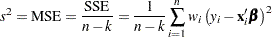 |
where  is the
  th row of the design matrix
  . The residual variance estimate is also unbiased:
  .
.
The covariance matrix of the least squares estimators is
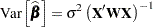 |
An estimate of the covariance matrix is obtained by replacing  with its estimate,
  in the preceding formula. This estimate is often referred to as COVB in SAS/STAT modeling procedures:
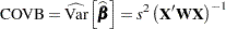 |
The correlation matrix of the estimates, often referred to as CORRB, is derived by scaling the covariance matrix: Let 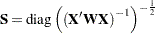 . Then the correlation matrix of the estimates is
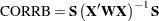 |
The estimated standard error of the th parameter estimator is obtained as the square root of the th diagonal element of the COVB matrix. Formally,
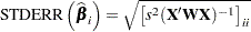 |
The ratio
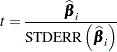 |
follows a Student’s distribution with  degrees of freedom under the hypothesis that
  is zero and provided that the model errors are normally distributed.
Regression procedures display the ratio and the significance probability, which is the probability under the hypothesis  of a larger absolute value than was actually obtained. When the probability is less than some small level, the event is considered so unlikely that the hypothesis is rejected.
Type I SS and Type II SS measure the contribution of a variable to the reduction in SSE. Type I SS measure the reduction in SSE as that variable is entered into the model in sequence. Type II SS are the increment in SSE that results from removing the variable from the full model. Type II SS are equivalent to the Type III and Type IV SS reported in the GLM procedure. If Type II SS are used in the numerator of an test, the test is equivalent to the test for the hypothesis that the parameter is zero. In polynomial models, Type I SS measure the contribution of each polynomial term after it is orthogonalized to the previous terms in the model. The four types of SS are described in
Chapter 15,
The Four Types of Estimable Functions.
Coefficient of Determination
The coefficient of determination in a regression model, also known as the R-square statistic ( ), measures the proportion of variability in the response that is explained by the regressor variables. In a linear regression model with intercept, is defined as
 |
where SSE is the residual (error) sum of squares and SST is the total sum of squares corrected for the mean. The adjusted statistic is an alternative to that takes into account the number of parameters in the model. This statistic is calculated as
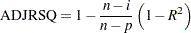 |
where  is the number of observations used to fit the model,
  is the number of parameters in the model (including the intercept), and is 1 if the model includes an intercept term, and 0 otherwise.
statistics also play an important indirect role in regression calculations. For example, the proportion of variability explained by regressing all other variables in a model on a particular regressor can provide insights into the interrelationship among the regressors.
Tolerances and variance inflation factors measure the strength of interrelationships among the regressor variables in the model. If all variables are orthogonal to each other, both tolerance and variance inflation are 1. If a variable is very closely related to other variables, the tolerance approaches 0 and the variance inflation gets very large. Tolerance (TOL) is 1 minus the that results from the regression of the other variables in the model on that regressor. Variance inflation (VIF) is the diagonal of  , if
, if  is scaled to correlation form. The statistics are related as
 |
Explicit and Implicit Intercepts
A linear model contains an explicit intercept if the matrix contains a column whose nonzero values do not vary, typically a column of ones. Many SAS/STAT procedures automatically add this column of ones as the first column in the matrix. Procedures that support a NOINT option in the MODEL statement provide the capability to suppress the automatic addition of the intercept column.
In general, models without intercept should be the exception, especially if your model does not contain classification variables. An overall intercept is provided in many models to adjust for the grand total or overall mean in your data. A simple linear regression without intercept, such as
 |
assumes that  has mean zero if
  takes on the value zero. This might not be a reasonable assumption.
If you explicitly suppress the intercept in a statistical model, the calculation and interpretation of your results can change. For example, the exclusion of the intercept in the following PROC REG statements leads to a different calculation of the R-square statistic. It also affects the calculation of the sum of squares in the analysis of variance for the model. For example, the model and error sum of squares add up to the uncorrected total sum of squares in the absence of an intercept.
proc reg;
   model y = x / noint;
quit;
Many statistical models contain an implicit intercept. This occurs when a linear function of one or more columns in the matrix produces a column of constant, nonzero values. For example, the presence of a CLASS variable in the GLM parameterization always implies an intercept in the model. If a model contains an implicit intercept, adding an intercept to the model does not alter the quality of the model fit, but it changes the interpretation (and number) of the parameter estimates.
The way in which the implicit intercept is detected and accounted for in the analysis depends on the procedure. For example, the following statements in the GLM procedure lead to an implied intercept:
proc glm;
   class a;
   model y = a / solution noint;
run;
Whereas the analysis of variance table uses the uncorrected total sum of squares (due to the NOINT option), the implied intercept does not lead to a redefinition or recalculation of the R-square statistic (compared to the model without the NOINT option). Also, because the intercept is implied by the presence of the CLASS variable a in the model, the same error sum of squares results whether the NOINT option is specified or not.
A different approach is taken, for example, by the TRANSREG procedure. The ZERO=NONE option in the CLASS parameterization of the following statements leads to an implicit intercept model:
proc transreg;
   model ide(y) = class(a / zero=none) / ss2;
run;
The analysis of variance table or the regression fit statistics are not affected in the TRANSREG procedure. Only the interpretation of the parameter estimates changes because of the way in which the intercept is accounted for in the model.
Implied intercepts not only occur when classification effects are present in the model. They also occur with B-splines and other sets of constructed columns.
Models Not of Full Rank
If the matrix is not of full rank, then a generalized inverse can be used to solve the normal equations to minimize the SSE:
 |
However, these estimates are not unique since there are an infinite number of solutions corresponding to different generalized inverses. PROC REG and other regression procedures choose a nonzero solution for all variables that are linearly independent of previous variables and a zero solution for other variables. This corresponds to using a generalized inverse in the normal equations, and the expected values of the estimates are the Hermite normal form of  multiplied by the true parameters:
 |
Degrees of freedom for the estimates that correspond to singularities are not counted (reported as zero). The hypotheses that are not testable have tests displayed as missing. The message that the model is not of full rank includes a display of the relations that exist in the matrix.
See the sections Generalized Inverse Matrices and Linear Model Theory in Chapter 3, Introduction to Statistical Modeling with SAS/STAT Software, on the nature and construction of generalized inverses and their importance for statistical inference in linear models.
Copyright © SAS Institute, Inc. All Rights Reserved.