PROC GLIMMIX: Maximum Likelihood Estimation Based on Adaptive Quadrature

The GLIMMIX Procedure

Maximum Likelihood Estimation Based on Adaptive Quadrature

Quadrature methods, like the Laplace approximation, approximate integrals. If you choose METHOD=QUAD for a generalized linear mixed model, the GLIMMIX procedure approximates the marginal log likelihood with an adaptive Gauss-Hermite quadrature rule. Gaussian quadrature is particularly well suited to numerically evaluate integrals against probability measures (Lange 1999, Ch. 16). And Gauss-Hermite quadrature is appropriate when the density has kernel $\text{[math]}$ and integration extends over the real line, as is the case for the normal distribution. Suppose that $\text{[math]}$ is a probability density function and the function $\text{[math]}$ is to be integrated against it. Then the quadrature rule is

$\text{[math]}$

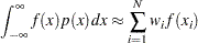where $\text{[math]}$ denotes the number of quadrature points, the $\text{[math]}$ are the quadrature weights, and the $\text{[math]}$ are the abscissas. The Gaussian quadrature chooses abscissas in areas of high density, and if $\text{[math]}$ is continuous, the quadrature rule is exact if $\text{[math]}$ is a polynomial of up to degree $\text{[math]}$ . In the generalized linear mixed model the roles of $\text{[math]}$ and $\text{[math]}$ are played by the conditional distribution of the data given the random effects, and the random-effects distribution, respectively. Quadrature abscissas and weights are those of the standard Gauss-Hermite quadrature (Golub and Welsch 1969; see also Table 25.10 of Abramowitz and Stegun 1972; Evans 1993).

A numerical integration rule is called adaptive when it uses a variable step size to control the error of the approximation. For example, an adaptive trapezoidal rule uses serial splitting of intervals at midpoints until a desired tolerance is achieved. The quadrature rule in the GLIMMIX procedure is adaptive in the following sense: if you do not specify the number of quadrature points (nodes) with the QPOINTS= suboption of the METHOD=QUAD option, then the number of quadrature points is determined by evaluating the log likelihood at the starting values at a successively larger number of nodes until a tolerance is met (for more details see the text under the heading "Starting Values" in the next section). Furthermore, the GLIMMIX procedure centers and scales the quadrature points by using the empirical Bayes estimates (EBEs) of the random effects and the Hessian (second derivative) matrix from the EBE suboptimization. This centering and scaling improves the likelihood approximation by placing the abscissas according to the density function of the random effects. It is not, however, adaptiveness in the previously stated sense.

Objective Function

Let $\text{[math]}$ denote the vector of fixed-effects parameters and $\text{[math]}$ the vector of covariance parameters. For quadrature estimation in the GLIMMIX procedure, $\text{[math]}$ includes the G-side parameters and a possible scale parameter $\text{[math]}$ , provided that the conditional distribution of the data contains such a scale parameter. $\text{[math]}$ is the vector of the G-side parameters. The marginal distribution of the data for subject $\text{[math]}$ in a mixed model can be expressed as

$\text{[math]}$

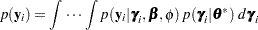Suppose $\text{[math]}$ denotes the number of quadrature points in each dimension (for each random effect) and $\text{[math]}$ denotes the number of random effects. For each subject, obtain the empirical Bayes estimates of $\text{[math]}$ as the vector $\text{[math]}$ that minimizes

$\text{[math]}$

If $\text{[math]}$ are the standard abscissas for Gauss-Hermite quadrature, and 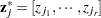$\text{[math]}$ is a point on the $\text{[math]}$ -dimensional quadrature grid, then the centered and scaled abscissas are

$\text{[math]}$

As for the Laplace approximation, $\text{[math]}$ is the second derivative matrix with respect to the random effects,

$\text{[math]}$

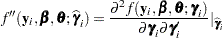These centered and scaled abscissas, along with the Gauss-Hermite quadrature weights $\text{[math]}$ , are used to construct the $\text{[math]}$ -dimensional integral by a sequence of one-dimensional rules

	$\text{[math]}$	$\text{[math]}$
	$\text{[math]}$	$\text{[math]}$
	$\text{[math]}$	$\text{[math]}$

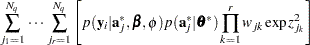The right-hand side of this expression, properly accumulated across subjects, is the objective function for adaptive quadrature estimation in the GLIMMIX procedure.

Quadrature or Laplace Approximation

If you select the quadrature rule with a single quadrature point, namely

proc glimmix method=quad(qpoints=1);

the results will be identical to METHOD=LAPLACE. Computationally, the two methods are not identical, however. METHOD=LAPLACE can be applied to a considerably larger class of models. For example, crossed random effects, models without subjects, or models with non-nested subjects can be handled with the Laplace approximation but not with quadrature. Furthermore, METHOD=LAPLACE draws on a number of computational simplifications that can increase its efficiency compared to a quadrature algorithm with a single node. For example, the Laplace approximation is possible with unbounded covariance parameter estimates (NOBOUND option in the PROC GLIMMIX statement) and can permit certain types of negative definite or indefinite $\text{[math]}$ matrices. The adaptive quadrature approximation with scaled abscissas typically breaks down when $\text{[math]}$ is not at least positive semidefinite.

As the number of random effects grows—for example, if you have nested random effects—quadrature quickly becomes computationally infeasible, due to the high dimensionality of the integral. To this end it is worthwhile to clarify the issues of dimensionality and computational effort as related to the number of quadrature nodes. Suppose that the A effect has 4 levels and consider the following statements:

proc glimmix method=quad(qpoints=5);
   class A id;
   model y = / dist=negbin;
   random A / subject=id;
run;

For each subject, computing the marginal log likelihood requires the numerical evaluation of a four-dimensional integral. As part of this evaluation $\text{[math]}$ conditional log likelihoods need to be computed for each observation on each pass through the data. As the number of quadrature points or the number of random effects increases, this constitutes a sizable computational effort. Suppose, for example, that an additional random effect with $\text{[math]}$ levels is added as an interaction. The following statements then require evaluation of $\text{[math]}$ conditional log likelihoods for each observation one each pass through the data:

proc glimmix method=quad(qpoints=5);
   class A B id;
   model y = / dist=negbin;
   random A A*B / subject=id;
run;

As the number of random effects increases, Laplace approximation presents a computationally more expedient alternative.

If you wonder whether METHOD=LAPLACE would present a viable alternative to a model that you can fit with METHOD=QUAD, the "Optimization Information" table can provide some insights. The table contains as its last entry the number of quadrature points determined by PROC GLIMMIX to yield a sufficiently accurate approximation of the log likelihood (at the starting values). In many cases, a single quadrature node is sufficient, in which case the estimates are identical to those of METHOD=LAPLACE.

Top of Page