| The NLMIXED Procedure |
| Active Set Methods |
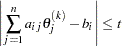
The parameter vector  can be subject to a set of
  linear equality and inequality constraints:
 |
 |
|||
 |
 |
The coefficients  and right-hand sides
  of the equality and inequality constraints are collected in the
  matrix
  and the vector
  .
.
The linear constraints define a feasible region  in
in  that must contain the point
  that minimizes the problem. If the feasible region is empty, no solution to the optimization problem exists.
In PROC NLMIXED, all optimization techniques use active set methods. The iteration starts with a feasible point  , which you can provide or which can be computed by the Schittkowski and Stoer (1979) algorithm implemented in PROC NLMIXED. The algorithm then moves from one feasible point
  to a better feasible point
  along a feasible search direction
  ,
,
 |
Theoretically, the path of points never leaves the feasible region of the optimization problem, but it can reach its boundaries. The active set  of point is defined as the index set of all linear equality constraints and those inequality constraints that are satisfied at . If no constraint is active , the point is located in the interior of , and the active set
  is empty. If the point in iteration
  hits the boundary of inequality constraint
  , this constraint becomes active and is added to . Each equality constraint and each active inequality constraint reduce the dimension (degrees of freedom) of the optimization problem.
In practice, the active constraints can be satisfied only with finite precision. The LCEPSILON= option specifies the range for active and violated linear constraints. If the point satisfies the condition
 |
where  , the constraint is recognized as an active constraint. Otherwise, the constraint is either an inactive inequality or a violated inequality or equality constraint. Due to rounding errors in computing the projected search direction, error can be accumulated so that an iterate steps out of the feasible region.
In those cases, PROC NLMIXED might try to pull the iterate back into the feasible region. However, in some cases the algorithm needs to increase the feasible region by increasing the LCEPSILON= value. If this happens, a message is displayed in the log output.
If the algorithm cannot improve the value of the objective function by moving from an active constraint back into the interior of the feasible region, it makes this inequality constraint an equality constraint in the next iteration. This means that the active set  still contains the constraint . Otherwise, it releases the active inequality constraint and increases the dimension of the optimization problem in the next iteration.
A serious numerical problem can arise when some of the active constraints become (nearly) linearly dependent. PROC NLMIXED removes linearly dependent equality constraints before starting optimization. You can use the LCSINGULAR= option to specify a criterion used in the update of the QR decomposition that determines whether an active constraint is linearly dependent relative to a set of other active constraints.
If the solution  is subjected to
  linear equality or active inequality constraints, the QR decomposition of the
  matrix
  of the linear constraints is computed by
  , where
  is an
is an  orthogonal matrix and
  is an upper triangular matrix. The
  columns of matrix can be separated into two matrices,
  , where
  contains the first orthogonal columns of and
  contains the last
  orthogonal columns of . The
  column-orthogonal matrix is also called the null-space matrix of the active linear constraints . The
  columns of the
  matrix form a basis orthogonal to the rows of the
  matrix
  .
.
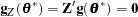
At the end of the iterating, PROC NLMIXED computes the projected gradient  ,
,
 |
In the case of boundary-constrained optimization, the elements of the projected gradient correspond to the gradient elements of the free parameters. A necessary condition for  to be a local minimum of the optimization problem is
 |
The symmetric  matrix
  ,
,
 |
is called a projected Hessian matrix. A second-order necessary condition for to be a local minimizer requires that the projected Hessian matrix is positive semidefinite.
Those elements of the vector of first-order estimates of Lagrange multipliers,
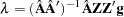 |
that correspond to active inequality constraints indicate whether an improvement of the objective function can be obtained by releasing this active constraint. For minimization, a significant negative Lagrange multiplier indicates that a possible reduction of the objective function can be achieved by releasing this active linear constraint. The LCDEACT= option specifies a threshold for the Lagrange multiplier that determines whether an active inequality constraint remains active or can be deactivated. (In the case of boundary-constrained optimization, the Lagrange multipliers for active lower (upper) constraints are the negative (positive) gradient elements corresponding to the active parameters.)
Copyright © 2009 by SAS Institute Inc., Cary, NC, USA. All rights reserved.