Gibbs Sampling

This section provides details about Bayesian analysis by Gibbs sampling in the location-scale models for survival data available in PROC LIFEREG. See the section Gibbs Sampler for a general discussion of Gibbs sampling. PROC LIFEREG fits parametric location-scale survival models. That is, the probability density of the response can expressed in the general form

where for lifetimes . The function determines the specific distribution. The location parameter is modeled through regression parameters as . The LIFEREG procedure can provide Bayesian estimates of the regression parameters and . The OUTPUT and PROBPLOT statements, if specified, are ignored. The PLOTS=PROBPLOT option in the PROC LIFEREG statement and the CORRB and COVB options in the MODEL statement are also ignored.

For the Weibull distribution, you can specify that Gibbs sampling be performed on the Weibull shape parameter instead of the scale parameter by specifying a prior distribution for the shape parameter with the WEIBULLSHAPEPRIOR= option. In addition, if there are no covariates in the model, you can specify Gibbs sampling on the Weibull scale parameter , where is the intercept term, with the WEIBULLSCALEPRIOR= option.

In the case of the exponential distribution with no covariates, you can specify Gibbs sampling on the exponential scale parameter , where is the intercept term, with the EXPSCALEPRIOR= option.

Let be the parameter vector. For location-scale models, the ’s are the regression coefficients ’s and the scale parameter . In the case of the three-parameter gamma distribution, there is an additional gamma shape parameter . Let be the likelihood function, where is the observed data. Let be the prior distribution. The full conditional distribution of is proportional to the joint distribution; that is,

For instance, the one-dimensional conditional distribution of given , is computed as

Suppose you have a set of arbitrary starting values . Using the ARMS (adaptive rejection Metropolis sampling) algorithm of Gilks and Wild (1992) and Gilks, Best, and Tan (1995), you can do the following:

• draw from

• draw from

• 

• draw from

This completes one iteration of the Gibbs sampler. After one iteration, you have . After iterations, you have . PROC LIFEREG implements the ARMS algorithm based on a program provided by Gilks (2003) to draw a sample from a full conditional distribution. See the section Assessing Markov Chain Convergence for information about assessing the convergence of the chain of posterior samples.

You can output these posterior samples into a SAS data set. The following option in the BAYES statement outputs the posterior samples into the SAS data set Post:

OUTPOST=Post

The data set also includes the variable LogPost, representing the log of the posterior log likelihood.

Priors for Model Parameters

The model parameters are the regression coefficients and the dispersion parameter (or the precision or scale), if the model has one. The priors for the dispersion parameter and the priors for the regression coefficients are assumed to be independent, while you can have a joint multivariate normal prior for the regression coefficients.

Scale and Shape Parameters

Gamma Prior

The gamma distribution has a pdf

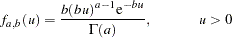where is the shape parameter and is the inverse-scale parameter. The mean is and the variance is .

Improper Prior

The joint prior density is given by

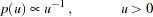Regression Coefficients

Let be the regression coefficients.

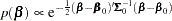
Normal Prior

Assume has a multivariate normal prior with mean vector and covariance matrix . The joint prior density is given by

Uniform Prior

The joint prior density is given by

Posterior Distribution

Denote the observed data by .

The posterior distribution is

where is the likelihood function with regression coefficients and any additional parameters, such as scale or shape, as parameters; and is the joint prior distribution of the parameters.

Deviance Information Criterion

Let be the model parameters at iteration of the Gibbs sampler, and let LL() be the corresponding model log likelihood. PROC LIFEREG computes the following fit statistics defined by Spiegelhalter et al. (2002):

• effective number of parameters:

• deviance information criterion (DIC):

where

and is the number of Gibbs samples.

Starting Values of the Markov Chains

When the BAYES statement is specified, PROC LIFEREG generates one Markov chain containing the approximate posterior samples of the model parameters. Additional chains are produced when the Gelman-Rubin diagnostics are requested. Starting values (or initial values) can be specified in the INITIAL= data set in the BAYES statement. If INITIAL= option is not specified, PROC LIFEREG picks its own initial values for the chains.

Denote as the integral value of x. Denote as the estimated standard error of the estimator .

Regression Coefficients and Gamma Shape Parameter

For the first chain that the summary statistics and regression diagnostics are based on, the default initial values are estimates of the mode of the posterior distribution. If the INITIALMLE option is specified, the initial values are the maximum likelihood estimates; that is,

Initial values for the th chain () are given by

with the plus sign for odd and minus sign for even .

Scale, Exponential Scale, Weibull Scale, or Weibull Shape Parameter

Let be the parameter sampled.

For the first chain that the summary statistics and diagnostics are based on, the initial values are estimates of the mode of the posterior distribution; or the maximum likelihood estimates if the INITIALMLE option is specified; that is,

The initial values of the th chain () are given by

with the plus sign for odd and minus sign for even .

OUTPOST= Output Data Set

The OUTPOST= data set contains the generated posterior samples. There are 2+ variables, where is the number of model parameters. The variable Iteration represents the iteration number and the variable LogPost contains the log posterior likelihood values. The other variables represent the draws of the Markov chain for the model parameters.