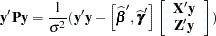
In computing the restricted likelihood function given previously, the determinants of the matrices and can be obtained effectively by using Cholesky decomposition. The quadratic term can be expressed in terms of solutions of mixed model equations as follows:

By default, the HPMIXED procedure profiles out the residual variance from the parameter vector . Let be the new parameter vector such that . The profiled objective function becomes

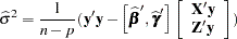
where and are the profiled versions of and , and are the ranks of and . Minimizing analytically for yields

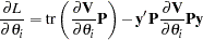
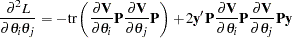
Optimizing the likelihood calls for derivatives with respect to the parameters. The first and second derivatives of the log-likelihood function with respect to scalar variance components and are

and

The default quasi-Newton method of optimization for the HPMIXED procedure requires only first derivatives of the log likelihood, and these are readily derived by solving the mixed model equations. For example, when , the first derivative of the log likelihood with respect to the parameter can be computed as follows:

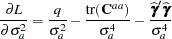where is the size of vector and is the part of the -inverse of the mixed model equation coefficient matrix corresponding to the random effect .

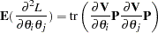
The second derivative of the log likelihood needs to be computed only if you specify certain nondefault optimization techniques in the NLOPTIONS statement, namely TECH=NEWRAP, TECH=NRRIDG, or TECH=TRUREG; see Nonlinear Optimization: The NLOPTIONS Statement in Chapter 18, Shared Concepts and Topics, for more information about optimization techniques. For these second-derivative-based optimization techniques, the HPMIXED procedure does not actually use the true second derivative matrix, or observed information matrix, as defined earlier. Instead, it uses an alternative matrix that is more efficient to compute for large problems and that can be more stable. This alternative is called the average information matrix, and it is defined as follows. The expected value of the second derivative is

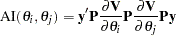
It is this trace that is computationally inefficient to evaluate. But if you average the expected information matrix defined by this formula with the observed information matrix defined by the preceding formula for the true second derivative, then the trace term cancels, leaving just a quadratic expression in . This quadratic expression defines the average information (Johnson and Thompson; 1995) with respect to and :