| The DISTANCE Procedure |
| Proximity Measures |
The following notation is used in this section:

the number of variables or the dimensionality

data for observation
 and the
  th variable, where

data for observation
 and the th variable, where
weight for the
th variable from the WEIGHTS= option in the VAR statement.  when either or is missing.
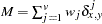
the sum of total weights. No matter if the observation is missing or not, its weight is added to this metric.

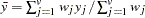
mean for observation
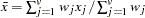

mean for observation

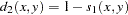
the distance or dissimilarity between observations
and 
the similarity between observations
and
The factor  is used to adjust some of the proximity measures for missing values.
Methods Accepting All Measurement Levels
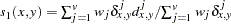
 is computed as follows:


Methods Accepting Ratio, Interval, and Ordinal Variables
- EUCLID
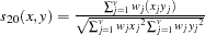
- SQEUCLID
- SIZE
- SHAPE
Note:squared shape distance plus squared size distance equals squared Euclidean distance.
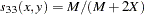
- COV
covariance similarity coefficient
 , where


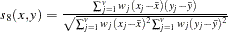
- CORR
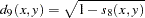
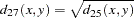
- DCORR
correlation transformed to Euclidean distance as sqrt(1–CORR)
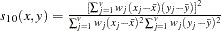
- SQCORR
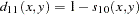
- DSQCORR
squared correlation transformed to squared Euclidean distance as (1–SQCORR)
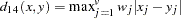
- L(
 )
) Minkowski (
 ) distance, where is a positive numeric value
- CITYBLOCK
- CHEBYCHEV
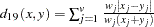
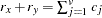
- POWER(
 )
) generalized Euclidean distance, where
is a nonnegative numeric value and  is a positive numeric value. The distance between two observations is the th root of sum of the absolute differences to the th power between the values for the observations:


Methods Accepting Ratio Variables
- SIMRATIO
- DISRATIO
- NONMETRIC
- CANBERRA
Canberra metric coefficient. See Sneath and Sokal (1973), pp. 125–126.
- COSINE
- DOT
- OVERLAP
- DOVERLAP
- CHISQ
chi-squared
If the data represent the frequency counts, chi-squared dissimilarity between two sets of frequencies can be computed. A 2-by- contingency table is illustrated to explain how the chi-squared dissimilarity is computed as follows: Variable
Row
Observation
Var 1
Var 2
...
Var v
Sum
X


...


Y


...


Column Sum


...


where


The chi-squared measure is computed as follows:

where for
= 1, 2, ..., 


- CHI
- PHISQ
phi-squared
This is the CHISQ dissimilarity normalized by the sum of weights
- PHI


Methods Accepting Symmetric Nominal Variables
The following notation is used for computing  to
to  . Notice that only the nonmissing pairs are discussed below; all the pairs with at least one missing value will be excluded from any of the computations in the following section because

nonmissing matches
 , where


nonmissing mismatches
 , where


total nonmissing pairs

- HAMMING
- MATCH
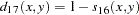
- DMATCH
simple matching coefficient transformed to Euclidean distance

- DSQMATCH
simple matching coefficient transformed to squared Euclidean distanc

- HAMANN
- RT
- SS1
- SS3
Sokal and Sneath 3. The coefficient between an observation and itself is always indeterminate (missing) since there is no mismatch.


The following notation is used for computing  to
to  . Notice that only the nonmissing pairs are discussed in the following section; all the pairs with at least one missing value are excluded from any of the computations in the following section because
Also, the observed nonmissing data of an asymmetric binary variable can have only two possible outcomes: presence or absence. Therefore, the notation, PX (present mismatches), always has a value of zero for an asymmetric binary variable.
The following methods distinguish between the presence and absence of attributes.
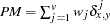
mismatches with at least one present
, where 


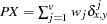
present matches
 , where


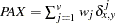
present mismatches
 , where

both present =


at least one present =


present-absent mismatches
 , where


total nonmissing pairs
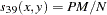
Methods Accepting Asymmetric Nominal and Ratio Variables
- JACCARD
Jaccard similarity coefficient
The JACCARD method is equivalent to the SIMRATIO method if there are only ratio variables; if there are both ratio and asymmetric nominal variables, the coefficient is computed as sum of the coefficient from the ratio variables (SIMRATIO) and the coefficient from the asymmetric nominal variables.

- DJACCARD
Jaccard dissimilarity coefficient
The DJACCARD method is equivalent to the DISRATIO method if there are only ratio variables; if there are both ratio and asymmetric nominal variables, the coefficient is computed as sum of the coefficient from the ratio variables (DISRATIO) and the coefficient from the asymmetric nominal variables.

Methods Accepting Asymmetric Nominal Variables
- DICE
Dice coefficient or Czekanowski/Sorensen similarity coefficient

- RR
Russell and Rao. This is the binary equivalent of the dot product coefficient.
- BLWNM
- BRAYCURTIS
Binary Lance and Williams, also known as Bray and Curtis coefficient

- K1
Kulcynski 1. The coefficient between an observation and itself is always indeterminate (missing) since there is no mismatch.
Copyright © 2009 by SAS Institute Inc., Cary, NC, USA. All rights reserved.