PROC CALIS: Longitudinal Factor Analysis :: SAS/STAT(R) 9.2 User's Guide, Second Edition

The CALIS Procedure

Example 25.6 Longitudinal Factor Analysis

The following example (McDonald 1980) illustrates both the ability of PROC CALIS to formulate complex covariance structure analysis problems by the generalized COSAN matrix model and the use of programming statements to impose nonlinear constraints on the parameters. The example is a longitudinal factor analysis that uses the Swaminathan (1974) model. For $\text{[math]}$ tests, $\text{[math]}$ occasions, and $\text{[math]}$ factors the matrix model is formulated in the section First-Order Autoregressive Longitudinal Factor Model as follows:

$\text{[math]}$

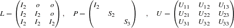
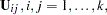The Swaminathan longitudinal factor model assumes that the factor scores for each ( $\text{[math]}$ ) common factor change from occasion to occasion ( $\text{[math]}$ ) according to a first-order autoregressive scheme. The matrix $\text{[math]}$ contains the $\text{[math]}$ factor loading matrices $\text{[math]}$ (each is $\text{[math]}$ ). The matrices $\text{[math]}$ and $\text{[math]}$ are diagonal, and the matrices $\text{[math]}$ and $\text{[math]}$ are subjected to the constraint

$\text{[math]}$

Since the constructed correlation matrix given by McDonald (1980) is singular, only unweighted least squares estimates can be computed. The following statements specify the COSAN model for the correlation structures.

   data Mcdon(TYPE=CORR);
   Title "Swaminathan's Longitudinal Factor Model, Data: McDONALD(1980)";     
   Title2 "Constructed Singular Correlation Matrix, GLS & ML not possible";   
      _TYPE_ = 'CORR'; INPUT _NAME_ $ Obs1-Obs9;                              
      datalines;                                                              
   Obs1  1.000    .      .      .      .      .      .      .      .          
   Obs2   .100  1.000    .      .      .      .      .      .      .          
   Obs3   .250   .400  1.000    .      .      .      .      .      .          
   Obs4   .720   .108   .270  1.000    .      .      .      .      .          
   Obs5   .135   .740   .380   .180  1.000    .      .      .      .          
   Obs6   .270   .318   .800   .360   .530  1.000    .      .      .          
   Obs7   .650   .054   .135   .730   .090   .180  1.000    .      .          
   Obs8   .108   .690   .196   .144   .700   .269   .200  1.000    .          
   Obs9   .189   .202   .710   .252   .336   .760   .350   .580  1.000        
        ;

   proc calis data=Mcdon method=ls tech=nr nobs=100;
   cosan B(6,Gen) * D1(6,Dia) * D2(6,Dia) * T(6,Low) * D3(6,Dia,Inv)
                  * D4(6,Dia,Inv) * P(6,Dia) + U(9,Sym);                      
      matrix B 
               [ ,1]= X1-X3,                                                  
               [ ,2]= 0. X4-X5,                                               
               [ ,3]= 3 * 0. X6-X8,                                           
               [ ,4]= 4 * 0. X9-X10,                                          
               [ ,5]= 6 * 0. X11-X13,                                         
               [ ,6]= 7 * 0. X14-X15;                                         
      matrix D1                                                                 
               [1,1]= 2 * 1. X16 X17 X16 X17;                                 
      matrix D2                                                                 
               [1,1]= 4 * 1. X18 X19;                                         
      matrix T                                                                  
               [1,1]= 6 * 1.,                                                 
               [3,1]= 4 * 1.,                                                 
               [5,1]= 2 * 1.;                                                 
      matrix D3                                                                 
               [1,1]= 4 * 1. X18 X19;                                         
      matrix D4                                                                 
               [1,1]= 2 * 1. X16 X17 X16 X17;                                 
      matrix P                                                                  
               [1,1]= 2 * 1. X20-X23;                                         
      matrix U                                                                  
               [1,1]= X24-X32,                                                
               [4,1]= X33-X38,                                                
               [7,1]= X39-X41;                                                
      bounds 0. <= X24-X32,                                                     
            -1. <= X16-X19 <= 1.;                                               
      X20 = 1. - X16 * X16;                                                     
      X21 = 1. - X17 * X17;                                                     
      X22 = 1. - X18 * X18;                                                     
      X23 = 1. - X19 * X19;                                                     
   run;

Because this formulation of Swaminathan’s model in general leads to an unidentified problem, the results given here are different from those reported by McDonald (1980). The displayed output of PROC CALIS also indicates that the fitted central model matrices $\text{[math]}$ and $\text{[math]}$ are not positive-definite. The BOUNDS statement constrains the diagonals of the matrices $\text{[math]}$ and $\text{[math]}$ to be nonnegative, but this cannot prevent $\text{[math]}$ from having three negative eigenvalues. The fact that many of the published results for more complex models in covariance structure analysis are connected to unidentified problems implies that more theoretical work should be done to study the general features of such models.

Top of Page