The HPPLS Procedure

Note that each extracted PLS factor is defined in terms of different X-variables ![]() . This leads to difficulties in comparing different scores, weights, and so on. The SIMPLS method of De Jong (1993) overcomes these difficulties by computing each score
. This leads to difficulties in comparing different scores, weights, and so on. The SIMPLS method of De Jong (1993) overcomes these difficulties by computing each score ![]() in terms of the original (centered and scaled) predictors
in terms of the original (centered and scaled) predictors ![]() . The SIMPLS X-weight vectors
. The SIMPLS X-weight vectors ![]() are similar to the eigenvectors of
are similar to the eigenvectors of ![]() , but they satisfy a different orthogonality condition. The
, but they satisfy a different orthogonality condition. The ![]() vector is just the first eigenvector
vector is just the first eigenvector ![]() (so that the first SIMPLS score is the same as the first PLS score). However, the second eigenvector maximizes
(so that the first SIMPLS score is the same as the first PLS score). However, the second eigenvector maximizes
whereas the second SIMPLS weight ![]() maximizes
maximizes
The SIMPLS scores are identical to the PLS scores for one response but slightly different for more than one response; see
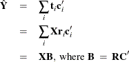
De Jong (1993) for details. The X- and Y-loadings are defined as in PLS, but because the scores are all defined in terms of ![]() , it is easy to compute the overall model coefficients
, it is easy to compute the overall model coefficients ![]() :
: