The server SQL Planner includes the STARJOIN facility. The server STARJOIN facility validates, optimizes, and executes SQL queries on data that is configured in a star schema. Star schemas consist of two or more normalized dimension tables that surround a centralized fact table. The centralized fact table contains data elements of interest, which are derived from the dimension tables.

In data warehouses with large numbers of tables and millions or billions of rows of data, a properly constructed star join can minimize overhead data redundancy during query evaluation. If the server STARJOIN facility is not enabled or if the server SQL does not detect a star schema, then the SQL is processed using pairwise joins.

A star join differs from a pairwise join in that in the server, a pairwise join requires one step for each table to complete the join. A properly configured star join requires only three steps to complete, regardless of the number of dimension tables. If a star schema consists of 25 dimension tables and one fact table, the star join is accomplished in three steps. But joining the tables in the star schema using pairwise joins requires 26 steps.

When data is configured in a valid server star schema, and the STARJOIN facility is not disabled, the server STARJOIN facility can produce quicker and more processor-efficient SQL query performance than SQL pairwise joins do.

Star Schemas

Overview of Star Schemas

To exploit the server STARJOIN facility, the data must be configured as a star schema, and it must meet specific server SQL star schema requirements.

Star schemas are the simplest data warehouse schema. They consist of a central fact table that is surrounded by multiple normalized dimension tables. Fact tables contain the measures of interest. Dimension tables provide detailed information about the attributes within each dimension. The columns that are in the fact tables are either foreign key columns that define the links between the fact table and individual dimension tables, or they are columns that calculate numeric values that are based on foreign key data.

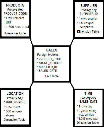
The following figure is an example star schema. The dimension tables Products, Supplier, Location, and Time surround the fact table Sales.

Example Star Schema

Diagram of a star schema with one fact table Sales and four dimension tables Products, Location, Time, Supplier

Example Dimension Tables Information

In the preceding figure, the Products table contains information about products, with one row per unique product SKU. The row for each unique SKU contains information such as product name, height, width, depth, weight, pallet cube, and so on. The Products table contains 1,500 rows.

The Supplier table contains information about the suppliers that supply the products. The row for each unique supplier contains information such as supplier name, address, state, contact representative, and so on. The Supplier table contains 25 rows.

The Location table contains information about the stores that sell the products. The row for each unique location contains information such as store number, store name, store address, store manager, store sales volume, and so on. The Location table contains 500 rows.

The Time table is a sequential sales transaction table. Each row in the Time table represents one day out of a rolling 3-year, 365-day-per-year calendar. The row for each day contains information such as the date, day of week, month, quarter, year, and so on. The table contains 1,095 rows.

Fact Table Information

The fact table, Sales, combines information from the four dimension tables (Products, Supplier, Location, and Time). Its foreign keys are imported, one from each dimension table: PRODUCT_CODE from Products, STORE_NUMBER from Location, SUPPLIER_ID from Supplier, and SALES_DATE from Time. The fact table Sales might have other columns that contain facts or information that is not found in any dimension table. Examples of fact table columns that are not foreign keys from a dimension table are columns such as QTY_SOLD or NET_SALES. The fact table in this example can contain as many as 1,500 x 25 x 500 x 1,095 = 20,531,250,000 rows.

Server STARJOIN Requirements

For the server SQL to take advantage of the STARJOIN Planner, the following conditions must be true:

STARJOIN optimization is enabled in the server.
The server star schema use a single, central fact table.
All dimension tables in the server star schema are connected to the fact table.
The server dimension tables appear in only one join condition.
The server fact tables are equally joined to dimension tables.
Dimension tables that do not use subsetting have a simple index on the dimension table's join column.

When you submit the server SQL that does not meet these STARJOIN conditions, the server performs the requested SQL task using the server's pairwise join strategy. For examples of valid, invalid, and restricted candidates for the server STARJOIN facility, see STARJOIN Examples.

Invoking the Server STARJOIN Facility

The server knows when to use the STARJOIN facility because of the topology of the data and the query. The server invokes STARJOIN based on the SQL that you submit. When you submit SQL and STARJOIN optimization is enabled, the server checks the SQL for admissible STARJOIN patterns. The server SQL identifies a fact table by scanning for a common, equally joined table among multiple join predicates in a WHERE clause. When the server SQL detects patterns that have multiple, equally joined operators that share a common table, the common table becomes the star schema's fact table.

When you submit an SQL statement to the server that uses structures that indicate the presence of a star schema, the STARJOIN validation checks begin.

Indexing Strategies to Optimize STARJOIN Query Performance

Overview of Indexing Strategies

When you have determined the baseline criteria for creating an SQL STARJOIN in the server, you can configure the indexes to influence which strategy the server STARJOIN facility chooses.

With the IN-SET strategy, the server STARJOIN facility can use multiple simple indexes on the fact table. The IN-SET strategy is the simplest to configure, and usually provides the best performance. To configure your indexes so that the STARJOIN facility chooses the IN-SET strategy, create a simple index on each SQL column in the fact table and dimension table that you want to use in a join relation. A simple index prevents STARJOIN Phase I from rejecting a Phase I dimension table so that it becomes a non-optimized Phase II table. Simple indexes also facilitate the Phase II fact-table-to-dimension-table join lookup.

Indexing to Optimize the IN-SET Join Strategy

Consider the following SQL code for a star schema with one fact table and two dimension tables:

proc sql;
select F.FID, D1.DKEY, D2.DKEY
from fact F, DIM1 D1, DIM2 D2
where D1.DKEY EQ F.D1KEY
and D2.DKEY EQ F.D2KEY
and D1.REGION EQ 'Midwest'
and D2.PRODUCT EQ 'TV';

The server IN-SET join strategy is the preferred strategy for almost every star join. If you want the example code to trigger the IN-SET STARJOIN strategy, create simple indexes on the join columns for the star schema's fact table and dimension tables:

On fact table F, create simple indexes on columns F.D1KEY and F.D2KEY.
On dimension tables D1 and D2, create simple indexes on columns D1.DKEY and D2.DKEY.

Other fact table and dimension table indexes might exist that could filter WHERE clauses. But the simple indexes are the indexes that will enable the STARJOIN IN-SET join strategy.

Indexing to Optimize the COMPOSITE Join Strategy

For the COMPOSITE join strategy, the dimension tables with WHERE clause subsetting are collected from the set of equally joined predicates. You need a composite index for the fact table columns that correspond to the subsetted dimension table columns. The composite index on the fact table is necessary to facilitate the dimension tables' Cartesian product probes on the fact table rows. The STARJOIN optimizer code looks for the best composite index, based on the best and simplest left-to-right match of the columns in the COMPOSITE join.

If the subsetting in a star join is limited to a single dimension table, then you can enable the COMPOSITE join strategy by creating a simple index on the join column of the single dimension table.

For the example code in Indexing to Optimize the IN-SET Join Strategy to trigger the COMPOSITE STARJOIN strategy, create a composite index named COMP1 on the fact table for each of the dimension table keys: F.COMP1=(D1KEY D2KEY).

Other fact table and dimension table indexes might exist that could filter WHERE clauses, but you need the COMPOSITE index named COMP1 in order to enable the STARJOIN COMPOSITE join strategy.

Although the COMPOSITE join strategy might appear to be a simpler configuration, the strongest utility of the COMPOSITE join strategy is limited to join relations between the fact table and dimension tables. As the number of dimension tables and join relations increases, the resulting increase in size can become unmanageable. The performance of the IN-SET strategy is robust enough that you should consider using the COMPOSITE join strategy only if you have good evidence that it compares favorably with the IN-SET strategy.

Example: Indexing Using the IN-SET Join Strategy

The example star schema in Example Star Schema has four dimension tables (Supplier, Products, Location, and Time) and one fact table (Sales). The schema has simple indexes on the SUPPLIER_ID, PRODUCT_CODE, STORE_NUMBER, and SALES_DATE columns in the Sales fact table.

Consider the following SQL query to create a January sales report for an organization's stores that are in North Carolina:

proc sql;
select
 sum(s.sales_amt) as sales_amt
 sum(s.units_sold) as units_sold
 s.product)code,
 t.sales_month

from
 spdslib.sales s,
 spdslib.supplier sup,
 spdslib.products p,
 spdslib.location l,
 spdslib.time t

where
 s.store_number = l.store_number
and s.sales_date = t.sales_date
and s.product_code = p.product_code
and s.supplier_id = sup.supplier_id
and l.state = 'NC'
and t.sales_date
 between '01JAN2015'd and '31JAN2015'd;

quit;

During optimization, the STARJOIN Planner examines the WHERE clause subsetting in the query to determine which dimension tables are processed first.

The WHERE clause subsetting of the STATE column of the Location dimension table (

where
                           ... l.state = 'NC'

) and the subsetting of the SALES_DATE column of the Time dimension table (

where ...
                           t.sales_date between '01JAN2015'd and '31JAN2015'd

) cause the server to process the Location and Time tables first. The remaining dimension tables, Supplier and Products, are processed second.

The server STARJOIN facility uses the first dimension tables to reduce the rows in the fact table to candidate rows that contain the matching criteria. The facility uses the values in each dimension table key to create a list of values that meet the subsetting criteria of the fact table.

For example, the previous SQL query is intended to create a January sales report for stores located in North Carolina. The WHERE clause in the SQL code joins the Location and Sales tables on the STORE_NUMBER column. Suppose that there are 10 unique North Carolina stores, with consecutively ordered STORE_NUMBER values that range from 101 to 110. When the WHERE clause is evaluated, the results will include a list of the 10 North Carolina store IDs that existed in January 2015.

Because the fact table and dimension tables for the STORE_NUMBER column have simple indexes, the STARJOIN facility chooses the IN-SET strategy. The facility subsets the STATE column values to 'NC' in order to build the set of store numbers that are associated with North Carolina locations. The STARJOIN facility can use the set of North Carolina store numbers to generate an SQL

where ...
                           in

expression. SQL uses the where ... in expression to efficiently subset the candidate rows in the fact table before the final SQL expression is evaluated.

Overview of STARJOIN Optimization

The server STARJOIN optimization process searches for the most efficient SQL strategy to use for computations. The STARJOIN optimization process consists of three steps, regardless of the number of dimension tables that are joined to the fact table in the star schema.

Classify dimension tables that are called by SQL as Phase I tables or Phase II tables.
Phase I of the process probes fact table indexes and selects a STARJOIN strategy.
Phase II of the process performs index lookups and joins subsetted fact table rows with Phase II tables.

Enabling STARJOIN Optimization

The server STARJOIN optimization is enabled by default. For information about statement options that enable or disable the STARJOIN facility in the server, see STARJOIN RESET Statement Options.

Classify Dimension Tables That Are Called by SQL as Phase I Tables or Phase II Tables

After the STARJOIN Planner validates the join subtree, join optimization begins. Join optimization is the process that searches for the most efficient SQL strategy to use to join the tables in the star schema.

The first step in the server’s join optimization is to examine the dimension tables that were called by SQL for structures that the server can use to improve performance. Each dimension table is classified as a Phase I table or a Phase II table. The structure of a dimension table and whether the SQL that you submit filters or subsets the table's contents determine its classification. The server uses different processes to handle Phase I and Phase II dimension tables.

Phase I tables can improve performance. A Phase I table is a dimension table that is either very small (nine rows or fewer), or a dimension table whose SQL queries contain one or more filtering criteria that are expressed with a WHERE clause. A Phase II table is any dimension table that does not meet Phase I criteria. Rows in Phase II tables that are referenced in the SQL query are not subsetted.

Consider the star schema that is shown in Example Star Schema, which contains the fact table Sales and the dimension tables Products, Supplier, Location, and Time.

Suppose that you submit an SQL query that requests transaction reports for all suppliers and for all products that meet the following criteria from the fact table Sales:

The store location is North Carolina.
The time period is the month of January.

The SQL query subsets the Location and Time tables, so the server classifies the Location and Time tables as Phase I tables. The query requests information from all of the rows in the Product and Supplier tables. Because those tables are not subsetted by a WHERE clause in the SQL, STARJOIN classifies the Products and Supplier tables in this query as Phase II tables.

Now, using the same star schema, add more detail to the SQL query. Set up a new query that requests transaction reports from the fact table Sales for all stores where the location is the state of North Carolina, for the month of January, and for products where the supplier is from the state of North Carolina. The subsetted dimension tables Location, Time, and Supplier are classified as Phase I tables. The Products table, unfiltered by the SQL query, is classified as a Phase II table.

Dimension tables are classified as Phase I or Phase II tables because the two types of tables require different index probe methods.

Phase I Probes Fact Table Indexes and Selects a STARJOIN Strategy

Phase I uses the SQL join keys from the subsetted Phase I dimension tables to get a smaller set of candidate rows to query in the central fact table. After the Phase I index probe optimizes the candidate rows in the fact table, the probe examines index structures to determine the best STARJOIN strategy to use. There are two server STARJOIN strategies: the IN-SET strategy and the COMPOSITE strategy. In all but a few cases, the IN-SET strategy is the most robust and efficient processing strategy. You can determine which strategy the server chooses by providing the required table index types in the SQL that you submit.

Phase I creates the smaller set of candidate rows in the central fact table by eliminating fact table rows that do not match the SQL join keys from the subsetted Phase I dimension tables. For example, if the SQL query requests information about transactions that occurred only in North Carolina store locations, the candidate rows that are retained in the fact table uses the SQL that subsets the Location dimension table:

WHERE location.STATE = "NC";

If the Sales fact table contains sales records for all 50 states, Phase I uses the SQL that subsets the Location dimension table to eliminate the sales records of all stores in states other than North Carolina from the fact table candidate rows. The fact table candidate rowset is reduced to transactions from only North Carolina stores, which eliminates massive amounts of nonproductive data processing.

The Phase I index probe inventories the number and types of indexes on the fact table and dimension tables as it attempts to identify the best STARJOIN strategy. To use the STARJOIN IN-SET strategy, Phase I must find simple indexes on all SQL join columns in the fact table and dimension tables. Otherwise, to use the STARJOIN COMPOSITE strategy, Phase I searches for the best composite index that is available on the fact table. The best composite index for the fact table is the composite index that spans the largest set of join predicates from the aggregated Phase I dimension tables.

Based on the fact table and dimension table index probe, the server selects the STARJOIN strategy by using the following logic:

If the probe finds one or more simple indexes on fact table and dimension table SQL join columns, and does not find spanning composite indexes on the fact table, the server selects the STARJOIN IN-SET strategy.
If the probe finds an optimal spanning composite index on the fact table, and does not find simple indexes on fact table and dimension table SQL join columns, the server selects the STARJOIN COMPOSITE strategy.
If the probe finds both simple and spanning composite indexes, the server generally selects the STARJOIN IN-SET strategy. If the composite index is an exact match for all of the Phase I join predicates, and only lesser matches are available with the IN-SET strategy, the server selects the IN-SET strategy.
If the probe does not find suitable indexes for either STARJOIN strategy, the server does not use STARJOIN. Instead, it joins the subtree using the standard server pairwise join.

The IN-SET and COMPOSITE join strategies have some underlying differences.

The IN-SET join strategy will cache temporary Phase 1 probes in memory, when possible, for use by Phase 2. The caching can result in significant performance improvements. By using in-memory lookups into the dimension tables for Phase 2 probes, rather than performing more costly file system probes of the dimension tables, significant performance improvements can result. The amount of memory allocated for Phase 1 IN-SET caching is controlled by the STARSIZE= server parameter. You can use the STARJOIN DETAILS option to see which partial results of the Phase 1 IN-SET strategy are cached, and whether sufficient memory was allocated for STARJOIN to cache all partial results.

The IN-SET join strategy uses an IN-SET transformation of dimension table metadata to produce a powerful compound WHERE clause to be used on the STARJOIN fact table. In the term IN-SET, IN refers to an IN specification in the SQL WHERE clause. The IN-SET is the set of values that populate the contents of the SQL IN query expression. For example, in the following SQL WHERE clause, the cities Raleigh, Cary, and Clayton are the values of the IN-SET:

WHERE location.CITY in ("Raleigh", "Cary", "Clayton");

For the IN-SET strategy, Phase I dimension tables are subsetted. Then the resulting set of join keys form the SQL IN expression for the fact table's corresponding join column. You must have simple indexes on all SQL join columns in both the fact table and dimension tables before STARJOIN Phase I can select the IN-SET strategy.

If the dimension table Location has six rows for Raleigh, Cary, and Clayton, then six STORE_NUMBER values are applied to the IN-SET WHERE clause that is used to select the candidate rows from the central fact table. The STARJOIN IN-SET facility transforms the dimension table's CITY values into STORE_NUMBER values that can be used to select candidate rows from the Sales fact table. The transformed WHERE clause that is applied to the fact table might resemble the following code:

WHERE fact.STORE_NUMBER in
 (100,101,102,103,104,105,106);

You can use IN-SET transformations in a star schema that has any number of dimension tables and a fact table. Consider the following example subsetting statement for a dimension table:

WHERE location.CITY in
("Raleigh","Cary","Clayton")
 and Time.SALES_WEEK = 1;

The Sales fact table has no matching CITY column to join with the Location dimension table, and no matching SALES_WEEK column to join with the Time table. Therefore, the IN-SET strategy uses transformations to create a WHERE clause that the Sales fact table can resolve:

WHERE fact.STORE_NUMBER in
 (100,101,102,103,104,105,106)
and Time.SALES_DATE in
 ('01JAN2015'd,'02JAN2015'd,'03JAN2015'd,
  '04JAN2015'd,'05JAN2015'd,'06JAN2015'd,
  '07JAN2015'd,);

The advantage of the STARJOIN facility is that it handles all of the transformations on a fact table, from dimension table subsetting to IN-SET WHERE clauses.

The COMPOSITE join strategy uses a composite index on the fact table to exhaustively probe the full Cartesian product of the combined join keys that is produced by the subsetting of the aggregated dimension table. The server compares the composite indexes on the fact table to the theoretical composite index that is made from all of the join keys in the Phase I dimension tables. Phase I selects the best composite index on the fact table, based on the join requirements of the dimension tables.

A disadvantage of using the COMPOSITE join strategy is that when more than a few join keys exist, the Cartesian product map can become large geometric matrices that can interfere with processing performance. You must have a composite index on the fact table that consists of Phase I dimension table join columns before STARJOIN Phase I can select the COMPOSITE join strategy.

If any Phase I dimension tables contain join predicates that do not have supporting simple or composite indexes on the fact table, those Phase I dimension tables are dropped from Phase I processing and are moved to the Phase II group.

Phase II Performs Index Lookups and Joins Subsetted Fact Table Rows with Phase II Tables

Phase I optimizes the join strategies between the Phase I dimension tables and the candidate rows from the fact table. After Phase I terminates, Phase II takes over. Phase II completes the indicated joins between the candidate rows from the fact table and the corresponding rows in the subsetted Phase I dimension tables. After Phase II completes the joins with the Phase I dimension tables, Phase II performs index lookups from the fact table to the Phase II dimension tables. For Phase II dimension tables, indexes should be created on all columns that join with the fact table.

When the server completes the STARJOIN Phase I and Phase II tasks, the STARJOIN optimizations have been performed, the STARJOIN strategy has been selected, and the subsetted dimension tables and fact table joins are ready to run and produce the SQL results set that you want.

Last updated: February 8, 2017