| The RELIABILITY Procedure |
| Regression Model Observation-wise Statistics |
For regression models that are fit using the MODEL statement, you can specify a variety of statistics to be computed for each observation in the input data set. This section describes the method of computation for each statistic. See Table 12.27 and Table 12.28 for the syntax for requesting these statistics.
Predicted Values
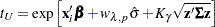
The linear predictor is
 |
where  is the vector of explanatory variables for the
  th observation.
Percentiles
An estimator of the  percentile
  for the th observation for the extreme value, normal, and logistic distributions is
 |
where  ,
,  is the standardized CDF, and
  is the distribution scale parameter.
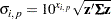
An estimator of the percentile  for the th observation for the Weibull, lognormal, and log-logistic distributions is
 |
where is the standardized CDF of the extreme value, normal, or logistic distribution that corresponds to the logarithm of the lifetime, and is the distribution scale parameter.
The percentile of the lognormal (base 10) distribution is
 |
where is the CDF of the standard normal distribution.
An estimator of the percentile for the th observation for the generalized gamma distribution is
 |
where
 |
and  is the percentile of the chi-square distribution with
  degrees of freedom.
Standard Errors of Percentile Estimator
For the extreme value, normal, and logistic distributions, the standard error of the estimator of the percentile is computed as
 |
where
 |
and  is the covariance matrix of
  .
.
For the Weibull, lognormal, and log-logistic distributions, the standard error is computed as
 |
where  is the percentile computed from the extreme value, normal, or logistic distribution that corresponds to the logarithm of the lifetime. The standard error for the lognormal (base 10) distribution is computed as
 |
The standard error for the generalized gamma distribution percentile is computed as
 |
where
 |
is the covariance matrix of  ,
,  is the vector of regression parameters, is the scale parameter, and
  is the shape parameter.
Confidence Limits for Percentiles
Two-sided approximate  confidence limits for for the extreme value, normal, and logistic distributions are computed as
 |
 |
 |
|||
 |
|
 |
where  represents the
  percentile of the standard normal distribution.
Limits for the Weibull, lognormal, and log-logistic percentiles are computed as
 |
|
 |
|||
 |
|
 |
where  and
and  are computed from the corresponding distributions for the logarithms of the lifetimes. For the lognormal (base 10) distribution,
|
|
 |
|||
|
|
 |
Limits for the generalized gamma distribution percentiles are computed as
 |
|||
 |
Reliability Function
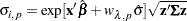
For the extreme value, normal, and logistic distributions, an estimate of the reliability function evaluated at the response  is computed as
 |
where  is the standardized CDF of the distribution from Table 12.60.
Estimates of the reliability function evaluated at the response  for the Weibull, lognormal, log-logistic, and generalized gamma distributions are computed as
 |
where is the standardized CDF of the corresponding extreme value, normal, logistic, or generalized log-gamma distributions.
Residuals
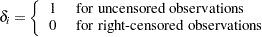
The RELIABILITY procedure computes several different kinds of residuals. In the following equations, represents the th response value if the extreme value, normal, or logistic distributions are specified. If is the th response and if the Weibull, lognormal, log-logistic, or generalized gamma distributions are specified, then represents the logarithm of the response  . If the lognormal (base 10) distribution is specified, then
  .
.
Raw Residuals
The raw residual is computed as
 |
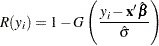
Standardized Residuals
The standardized residual is computed as
 |
Adjusted Residuals
If an observation is right censored, then the standardized residual for that observation is also right censored. Adjusted residuals adjust censored standardized residuals upward by adding a percentile of the residual lifetime distribution, given that the standardized residual exceeds the censoring value. The default percentile is the median (50th percentile), but you can, optionally, specify a  percentile by using the RESIDALPHA=
 option in the MODEL statement. The
  percentile residual life is computed as in Joe and Proschan (1984). The adjusted residual is computed as
 |
where is the standard CDF,
 |
is the reliability function, and
 |
If the generalized gamma distribution is specified, the standardized CDF and reliability functions include the estimated shape parameter  .
.
Modified Cox-Snell Residuals
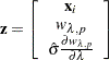
Let
 |
The Cox-Snell residual is defined as
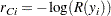 |
where
 |
is the reliability function. The modified Cox-Snell residual is computed as in Collett (1994, p. 152):
 |
where  is an adjustment factor. If the fitted model is correct, the Cox-Snell residual has approximately a standard exponential distribution for uncensored observations. If an observation is censored, the residual evaluated at the censoring time is not as large as the residual evaluated at the (unknown) failure time. The adjustment factor adjusts the censored residuals upward to account for the censoring. The default is
  , the median of the standard exponential distribution. You can, optionally, specify any adjustment factor by using the MODEL statement option RESIDADJ=. Another commonly used value is the mean of the standard exponential distribution,
  .
.


Copyright © SAS Institute, Inc. All Rights Reserved.