High-Performance Features of the OPTGRAPH Procedure
Example: Centrality by Cluster for a Simple Undirected Graph
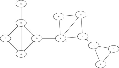
This example uses the same simple undirected graph as in the previous example; it is shown again in Figure 1.9. However, this example does not use community detection. Instead, the data set is manually predistributed by the cluster variable, where the cluster variable can define any partition of the nodes.
Figure 1.9: Undirected Graph
The following statements create the data set LinkSetIn:
data LinkSetIn;
   input from $ to $ @@;
   datalines;
A B  A C  A D  B C  C D
C E  D F  F G  F H  F I
G H  G I  I J  J K  J L
K L
;
The graph seems to have three distinct parts, which are connected by just a few links. Assume that you have already partitioned
the data set into three sets of nodes: ![]() ,
, ![]() , and
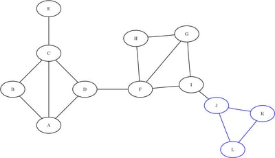
, and ![]() . The induced subgraphs on these three sets of nodes are shown in blue in Figure 1.10 through Figure 1.12.
. The induced subgraphs on these three sets of nodes are shown in blue in Figure 1.10 through Figure 1.12.
Figure 1.10: Subgraph ![]()
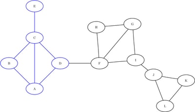
Figure 1.11: Subgraph ![]()
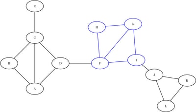
Figure 1.12: Subgraph ![]()
The following data sets define the three induced subgraphs:
data LinkSetIn0;
   input from $ to $ @@;
   datalines;
A B  A C  A D  B C  C D  C E
;

data LinkSetIn1;
   input from $ to $ @@;
   datalines;
F G  F H  F I  G H  G I
;

data LinkSetIn2;
   input from $ to $ @@;
   datalines;
J K  J L  K L
;
To calculate centrality metrics on the three subgraphs, you could run PROC OPTGRAPH three times, as follows:
proc optgraph
   data_links = LinkSetIn0
   out_nodes  = NodeSetOut0;
   centrality
      degree    = out
      influence = unweight
      close     = unweight
      between   = unweight
      eigen     = unweight;
run;

proc optgraph
   data_links = LinkSetIn1
   out_nodes  = NodeSetOut1;
   centrality
      degree    = out
      influence = unweight
      close     = unweight
      between   = unweight
      eigen     = unweight;
run;

proc optgraph
   data_links = LinkSetIn2
   out_nodes  = NodeSetOut2;
   centrality
      degree    = out
      influence = unweight
      close     = unweight
      between   = unweight
      eigen     = unweight;
run;
This produces the results shown in Figure 1.13 through Figure 1.15.
Figure 1.13: Centrality for Induced Subgraph 0
Figure 1.14: Centrality for Induced Subgraph 1
Figure 1.15: Centrality for Induced Subgraph 2
A much more efficient way to process these graphs is to use the BY_CLUSTER option. The section "Processing by Cluster" in SAS OPTGRAPH Procedure: Graph Algorithms and Network Analysis shows how to use the BY_CLUSTER option for running in single-machine mode. This example shows the same process for running in distributed mode.
Define the partitions of the original graph by adding a cluster variable to the links data set. This variable denotes the partition to which each link belongs. If the partition is defined
over nodes, then any links that span from one partition to another are removed from the input data set.
data LinkSetCluster;
   input from $ to $ cluster @@;
   datalines;
A B 0 A C 0 A D 0 B C 0 C D 0 C E 0
F G 1 F H 1 F I 1 G H 1 G I 1
J K 2 J L 2 K L 2
;
Next, use PROC HPDS2 to distribute the links data set to the appliance by cluster, as follows:
libname gplib greenplm
   server             = "grid001.example.com"
   schema             = public
   user               = dbuser
   password           = dbpass
   database           = hps
   preserve_col_names = yes;

proc datasets nolist lib=gplib;
   delete LinkSetIn;
run;

proc hpds2
   data = LinkSetIn
   out  = gplib.LinkSetIn (distributed_by='distributed by (cluster)');
   performance
      host    = "grid001.example.com"
      install = "/opt/TKGrid";
   data DS2GTF.out;
      method run();
         set DS2GTF.in;
      end;
   enddata;
run;
You use the LIBNAME option PRESERVE_COL_NAMES=YES because the links data set contains the variable from, which is a keyword reserved for DBMS tables that use SAS/ACCESS. (See
SAS/ACCESS for Relational Databases: Reference.)
Now, by using one call to PROC OPTGRAPH, you can process all three induced subgraphs on the appliance in parallel, as follows:
proc datasets nolist lib=gplib;
   delete NodeSetCentrality;
run;

proc optgraph
    data_links      = gplib.LinkSetCluster
    out_nodes       = gplib.NodeSetCentrality;
   performance
      host    = "grid001.example.com"
      install = "/opt/TKGrid";
    centrality
        by_cluster
        degree      = out
        influence   = unweight
        close       = unweight
        between     = unweight
        eigen       = unweight;
run;
In this example, the results in the data set that is specified by the OUT_NODES= option are stored in distributed form on
the appliance in gplib.NodeSetCentrality. For the sake of display, a local version of the data is created and sorted as follows:
data NodeSetCentrality;
   set gplib.NodeSetCentrality;
run;
proc sort data=NodeSetCentrality;
   by cluster descending centr_eigen_unwt;
run;
The results are shown in Figure 1.16.
Figure 1.16: Centrality for All Induced Subgraphs
| node | cluster | centr_degree_out | centr_eigen_unwt | centr_close_unwt | centr_between_unwt | centr_influence1_unwt | centr_influence2_unwt |
|---|---|---|---|---|---|---|---|
| C | 0 | 4 | 1.00000 | 1.00000 | 0.58333 | 0.80000 | 1.60000 |
| A | 0 | 3 | 0.89897 | 0.80000 | 0.08333 | 0.60000 | 1.60000 |
| D | 0 | 2 | 0.70711 | 0.66667 | 0.00000 | 0.40000 | 1.40000 |
| B | 0 | 2 | 0.70711 | 0.66667 | 0.00000 | 0.40000 | 1.40000 |
| E | 0 | 1 | 0.37236 | 0.57143 | 0.00000 | 0.20000 | 0.80000 |
| G | 1 | 3 | 1.00000 | 1.00000 | 0.16667 | 0.75000 | 1.75000 |
| F | 1 | 3 | 1.00000 | 1.00000 | 0.16667 | 0.75000 | 1.75000 |
| H | 1 | 2 | 0.78078 | 0.75000 | 0.00000 | 0.50000 | 1.50000 |
| I | 1 | 2 | 0.78078 | 0.75000 | 0.00000 | 0.50000 | 1.50000 |
| J | 2 | 2 | 1.00000 | 1.00000 | 0.00000 | 0.66667 | 1.33333 |
| K | 2 | 2 | 1.00000 | 1.00000 | 0.00000 | 0.66667 | 1.33333 |
| L | 2 | 2 | 1.00000 | 1.00000 | 0.00000 | 0.66667 | 1.33333 |