High-Performance Features of the OPTGRAPH Procedure

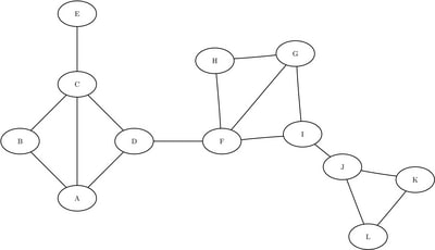
This section illustrates the use of the community detection algorithm in distributed mode on the simple undirected graph depicted in Figure 1.1.

Figure 1.1: A Simple Undirected Graph

The following statements create the data set LinkSetIn:

data LinkSetIn;
   input from $ to $ @@;
   datalines;
A B  A C  A D  B C  C D
C E  D F  F G  F H  F I
G H  G I  I J  J K  J L
K L
;

Before you run community detection in distributed mode, you must convert the undirected graph to a directed graph by replicating links in both directions, as shown in the following statements:

data LinkSetIn;
   set LinkSetIn;
   output;
   tmp  = from;
   from = to;
   to   = tmp;
   output;
   drop tmp;
run;

Then you can use PROC HPDS2 to distribute the links data to the appliance by from as follows:

libname gplib greenplm
   server            = "grid001.example.com"
   schema            = public
   user              = dbuser
   password          = dbpass
   database          = hps
   preserve_col_names=yes;

proc datasets nolist lib=gplib;
   delete LinkSetIn;
quit;

proc hpds2
   data = LinkSetIn
   out  = gplib.LinkSetIn (distributed_by='distributed by (from)');
   performance
      host    = "grid001.example.com"
      install = "/opt/TKGrid";
   data DS2GTF.out;
      method run();
         set DS2GTF.in;
      end;
   enddata;
run;

The LIBNAME statement option PRESERVE_COL_NAMES=YES is used because the links data set contains the variable from, which is a reserved keyword for DBMS tables that use SAS/ACCESS. For more information, see SAS/ACCESS for Relational Databases: Reference.

After the data have been distributed to the appliance, you can invoke PROC OPTGRAPH. In this example, some of the output data sets are written to the appliance and other output data sets are written to the client machine. It is recommended that the large output data sets be stored in the DBMS, because transferring data from the appliance to the client machine can take a very long time. In addition, further analysis (such as centrality computation) can benefit from the data’s already being distributed on the appliance. In the following statements, CommLevelOut and CommOut are stored on the client machine in the WORK library, and the remaining output data sets are stored on the appliance, although the output data sets for this simple example are very small:

proc datasets nolist lib=gplib;
   delete NodeSetOut CommOverlapOut CommLinksOut CommIntraLinksOut;
quit;

proc optgraph
   graph_direction = directed
   data_links      = gplib.LinkSetIn
   out_nodes       = gplib.NodeSetOut;
   performance
      host    = "grid001.example.com"
      install = "/opt/TKGrid";
   community
      resolution_list      = 0.001
      algorithm            = parallel_label_prop
      out_level            = CommLevelOut
      out_community        = CommOut
      out_overlap          = gplib.CommOverlapOut
      out_comm_links       = gplib.CommLinksOut
      out_intra_comm_links = gplib.CommIntraLinksOut;
run;

The data set NodeSetOut contains the community identifier of each node. It is shown in Figure 1.2.

The data set CommLevelOut contains the number of communities and the corresponding modularity values that are found at each resolution level. It is shown in Figure 1.3.

The data set CommOut contains the number of nodes that are contained in each community. It is shown in Figure 1.4.

The data set CommOverlapOut contains the intensity of each node that belongs to multiple communities. It is shown in Figure 1.5. In this example, node F is connected to two communities, with 75% of its links connecting to community 1 and 25% of its links connecting to community 2.

The data set CommLinksOut shows how the communities are interconnected. It is shown in Figure 1.6.

The data set CommIntraLinksOut shows how the nodes are connected within each community. It is shown in Figure 1.7.