The NETDRAW Procedure
- Overview
- Getting Started
-
Syntax

-
DetailsNetwork Input Data SetVariables in the Network Data SetMissing ValuesLayout of the NetworkFormat of the DisplayPage FormatLayout Data SetControlling the LayoutTime-Scaled Network DiagramsZoned Network DiagramsOrganizational Charts or Tree DiagramsFull-Screen VersionGraphics VersionUsing the Annotate FacilityWeb-Enabled Network DiagramsMacro Variable _ORNETDRComputer Resource RequirementsODS Style Templates
-
ExamplesLine-Printer Network DiagramGraphics Version of PROC NETDRAWSpanning Multiple PagesThe COMPRESS and PCOMPRESS OptionsControlling the Display FormatNonstandard Precedence RelationshipsControlling the Arc-Routing AlgorithmPATTERN and SHOWSTATUS OptionsTime-Scaled Network DiagramFurther Time-Scale OptionsZoned Network DiagramSchematic DiagramsModifying Network LayoutSpecifying Node PositionsOrganizational Charts with PROC NETDRAWAnnotate Facility with PROC NETDRAWAOA Network Using the Annotate FacilityBranch and Bound TreesStatement and Option Cross-Reference Tables
- References
The first step in defining a project is to make a list of the activities in the project and determine the precedence constraints
that need to be satisfied by these activities. It is useful at this stage to view a graphical representation of the project
network. In order to draw the network, you specify the nodes of the network and the precedence relationships among them. Consider
the software development project that is described in the “Getting Started” section of Chapter 4: The CPM Procedure. The network data are in the SAS data set SOFTWARE, displayed in Figure 9.1.
Figure 9.1: Software Project
| Software Project |
| Data Set SOFTWARE |
| Obs | descrpt | duration | activity | succesr1 | succesr2 |
|---|---|---|---|---|---|
| 1 | Initial Testing | 20 | TESTING | RECODE | |
| 2 | Prel. Documentation | 15 | PRELDOC | DOCEDREV | QATEST |
| 3 | Meet Marketing | 1 | MEETMKT | RECODE | |
| 4 | Recoding | 5 | RECODE | DOCEDREV | QATEST |
| 5 | QA Test Approve | 10 | QATEST | PROD | |
| 6 | Doc. Edit and Revise | 10 | DOCEDREV | PROD | |
| 7 | Production | 1 | PROD |
The following code produces the network diagram shown in Figure 9.2:
pattern1 v=e c=green;
pattern2 v=e c=red;

title h=3 'Software Project';
proc netdraw graphics data=software;
   actnet / act=activity htext=2
            succ=(succesr1 succesr2)
            pcompress separatearcs;
   run;
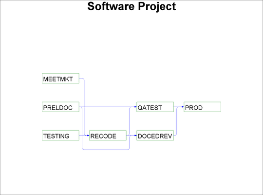
The procedure determines the placement of the nodes and the routing of the arcs on the basis of the topological ordering of
the nodes and attempts to produce a compact diagram. You can control the placement of the nodes by specifying explicitly the
node positions. The data set SOFTNET, shown in Figure 9.3, includes the variables _X_ and _Y_, which specify the desired node coordinates. Note that the precedence information is conveyed using a single SUCCESSOR variable
unlike the data set SOFTWARE, which contains two SUCCESSOR variables.
Figure 9.3: Software Project: Specify Node Positions
| Software Project |
| Data Set SOFTNET |
| Obs | descrpt | duration | activity | succesor | _x_ | _y_ |
|---|---|---|---|---|---|---|
| 1 | Initial Testing | 20 | TESTING | RECODE | 1 | 1 |
| 2 | Meet Marketing | 1 | MEETMKT | RECODE | 1 | 2 |
| 3 | Prel. Documentation | 15 | PRELDOC | DOCEDREV | 1 | 3 |
| 4 | Prel. Documentation | 15 | PRELDOC | QATEST | 1 | 3 |
| 5 | Recoding | 5 | RECODE | DOCEDREV | 2 | 2 |
| 6 | Recoding | 5 | RECODE | QATEST | 2 | 2 |
| 7 | QA Test Approve | 10 | QATEST | PROD | 3 | 3 |
| 8 | Doc. Edit and Revise | 10 | DOCEDREV | PROD | 3 | 1 |
| 9 | Production | 1 | PROD | 4 | 2 |
The following code produces a network diagram (shown in Figure 9.4) with the new node placement:
title h=3 'Software Project';
title2 h=2 'Controlled Layout';
proc netdraw graphics data=softnet;
   actnet / act=activity htext=1.25
            succ=(succesor)
            pcompress;
   run;
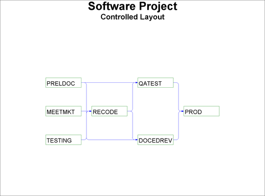
Figure 9.5: Software Project Schedule
| Software Project |
| Project Schedule |
| descrpt | activity | succesr1 | succesr2 | duration | E_START | E_FINISH | L_START | L_FINISH | T_FLOAT | F_FLOAT |
|---|---|---|---|---|---|---|---|---|---|---|
| Initial Testing | TESTING | RECODE | 20 | 01MAR04 | 20MAR04 | 01MAR04 | 20MAR04 | 0 | 0 | |
| Prel. Documentation | PRELDOC | DOCEDREV | QATEST | 15 | 01MAR04 | 15MAR04 | 11MAR04 | 25MAR04 | 10 | 10 |
| Meet Marketing | MEETMKT | RECODE | 1 | 01MAR04 | 01MAR04 | 20MAR04 | 20MAR04 | 19 | 19 | |
| Recoding | RECODE | DOCEDREV | QATEST | 5 | 21MAR04 | 25MAR04 | 21MAR04 | 25MAR04 | 0 | 0 |
| QA Test Approve | QATEST | PROD | 10 | 26MAR04 | 04APR04 | 26MAR04 | 04APR04 | 0 | 0 | |
| Doc. Edit and Revise | DOCEDREV | PROD | 10 | 26MAR04 | 04APR04 | 26MAR04 | 04APR04 | 0 | 0 | |
| Production | PROD | 1 | 05APR04 | 05APR04 | 05APR04 | 05APR04 | 0 | 0 |
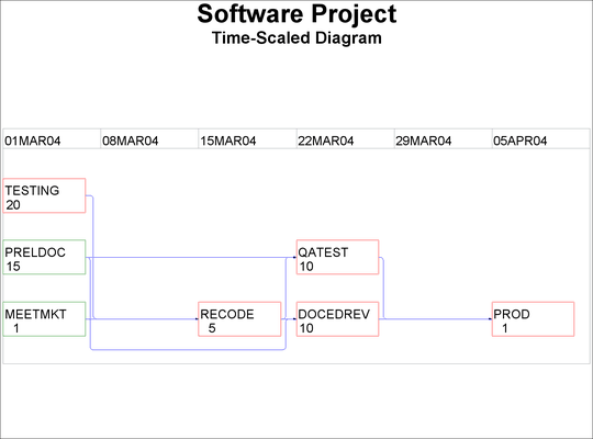
While the project is in progress, you may want to use the network diagram to show the current status of each activity as well
as any other relevant information about each activity. PROC NETDRAW can also be used to produce a time-scaled network diagram
using the schedule produced by PROC CPM. The schedule data for the software project described earlier are saved in a data
set, INTRO1, which is shown in Figure 9.5.
To produce a time-scaled network diagram, use the TIMESCALE option in the ACTNET statement, as shown in the following program. The MININTERVAL= and the LINEAR options are used to control the time axis on the diagram. The ID=, NOLABEL, and NODEFID options control the amount of information displayed within each node. The resulting diagram is shown in Figure 9.6.
title h=3 'Software Project';
title2 h=2 'Time-Scaled Diagram';
proc netdraw graphics data=intro1;
   actnet / act=activity succ=(succ:)
            separatearcs pcompress htext=2
            timescale linear frame mininterval=week
            id=(activity duration) nolabel nodefid;
   run;
Several other options are available to control the layout of the nodes, the appearance of the network, and the format of the time axis. For projects that have natural divisions, you can use the ZONE= option to divide the network into horizontal zones or bands. For networks that have an embedded tree structure, you can use the TREE option to draw the network like a tree laid out from left to right, with the root at the left edge of the diagram; in graphics mode, you can obtain a top-down tree with the root at the top of the diagram. For cyclic networks you can use the BREAKCYCLE option to enable the procedure to break cycles. All of these options are discussed in detail in the following sections.