The NETFLOW Procedure
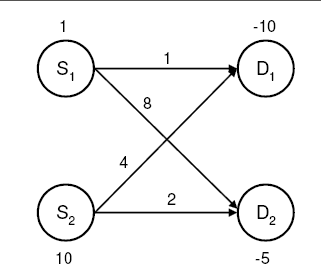
In this example we illustrate the use of the EXCESS= option for various scenarios in pure networks. Consider a simple network as shown in Output 6.9.1. The positive numbers on the nodes correspond to supply and the negative numbers correspond to demand. The numbers on the arcs indicate costs.
We first analyze a simple transportation problem where total demand exceeds total supply, as seen in Output 6.9.1. The EXCESS=SLACKS option is illustrated first.
The following SAS code creates the input data sets.
data parcs;
   input _from_ $ _to_ $ _cost_;
datalines;
s1 d1 1
s1 d2 8
s2 d1 4
s2 d2 2
;

data SleD;
   input _node_ $ _sd_;
datalines;
s1   1
s2  10
d1 -10
d2  -5
;
You can solve the problem using the following call to PROC NETFLOW:
title1 'The NETFLOW Procedure';
proc netflow
   excess   = slacks
   arcdata  = parcs
   nodedata = SleD
   conout   = solex1;
run;
Since the EXCESS=SLACKS option is specified, the interior point method is used for optimization. Accordingly, the CONOUT= data set is specified. The optimal solution is displayed in Output 6.9.2.
The solution with the THRUNET option specified is displayed in Output 6.9.3.
title1 'The NETFLOW Procedure';
proc netflow
   thrunet
   excess   = slacks
   arcdata  = parcs
   nodedata = SleD
   conout   = solex1t;
run;
Note: If you want to use the network simplex solver instead, you need to specify the EXCESS=ARCS option and, accordingly, the
ARCOUT= data set.
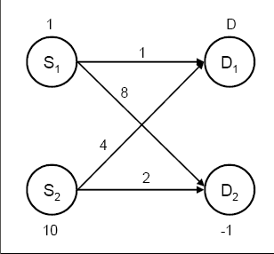
As shown in Output 6.9.4, node ![]() has a missing D demand value.
has a missing D demand value.
The following code creates the node data set:
data node_missingD1;
   input _node_ $ _sd_;
   missing D;
datalines;
s1   1
s2  10
d1   D
d2  -1
;
You can use the following call to PROC NETFLOW to solve the problem:
title1 'The NETFLOW Procedure';
proc netflow
   excess   = slacks
   arcdata  = parcs
   nodedata = node_missingD1
   conout   = solex1b;
run;
The optimal solution is displayed in Output 6.9.5. As you can see, the flow balance at nodes with nonmissing supdem values is maintained. In other words, if a node has a nonmissing supply (demand) value, then the sum of flows out of (into)
that node is equal to its supdem value.
Consider the previous example, but with the THRUNET option specified.
title1 'The NETFLOW Procedure';
proc netflow
   thrunet
   excess   = slacks
   arcdata  = parcs
   nodedata = node_missingD1
   conout   = solex1c;
run;
The optimal solution is displayed in Output 6.9.6. By specifying the THRUNET option, we have actually obtained the minimum-cost flow through the network, while maintaining flow balance at the nodes with nonmissing supply values.
Note: The case with missing S supply values is similar to the case with missing D demand values.