The NETFLOW Procedure
Consider the following trans-shipment problem for an oil company. Crude oil is shipped to refineries where it is processed into gasoline and diesel fuel. The gasoline and diesel fuel are then distributed to service stations. At each stage, there are shipping, processing, and distribution costs. Also, there are lower flow bounds and capacities.
In addition, there are two sets of side constraints. The first set is that two times the crude from the Middle East cannot exceed the throughput of a refinery plus 15 units. (The phrase "plus 15 units" that finishes the last sentence is used to enable some side constraints in this example to have a nonzero rhs.) The second set of constraints are necessary to model the situation that one unit of crude mix processed at a refinery yields three-fourths of a unit of gasoline and one-fourth of a unit of diesel fuel.
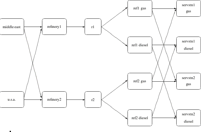
Because there are two products that are not independent in the way in which they flow through the network, a network programming problem with side constraints is an appropriate model for this example (see Figure 6.6). The side constraints are used to model the limitations on the amount of Middle Eastern crude that can be processed by each refinery and the conversion proportions of crude to gasoline and diesel fuel.
To solve this problem with PROC NETFLOW, save a representation of the model in three SAS data sets. In the NODEDATA= data set, you name the supply and demand nodes and give the associated supplies and demands. To distinguish demand nodes from supply nodes, specify demands as negative quantities. For the oil example, the NODEDATA= data set can be saved as follows:
title  'Oil Industry Example';
title3 'Setting Up Nodedata = Noded For Proc Netflow';
data noded;
  input   _node_&$15. _sd_;
  datalines;
middle east       100
u.s.a.             80
servstn1 gas      -95
servstn1 diesel   -30
servstn2 gas      -40
servstn2 diesel   -15
;
The ARCDATA= data set contains the rest of the information about the network. Each observation in the data set identifies an arc in the network and gives the cost per flow unit across the arc, the capacities of the arc, the lower bound on flow across the arc, and the name of the arc.
title3 'Setting Up Arcdata = Arcd1 For Proc Netflow';
data arcd1;
  input _from_&$11. _to_&$15. _cost_ _capac_ _lo_ _name_ $;
  datalines;
middle east    refinery 1        63     95   20    m_e_ref1
middle east    refinery 2        81     80   10    m_e_ref2
u.s.a.         refinery 1        55      .    .    .
u.s.a.         refinery 2        49      .    .    .
refinery 1     r1               200    175   50    thruput1
refinery 2     r2               220    100   35    thruput2
r1             ref1 gas           .    140    .    r1_gas
r1             ref1 diesel        .     75    .    .
r2             ref2 gas           .    100    .    r2_gas
r2             ref2 diesel        .     75    .    .
ref1 gas       servstn1 gas      15     70    .    .
ref1 gas       servstn2 gas      22     60    .    .
ref1 diesel    servstn1 diesel   18      .    .    .
ref1 diesel    servstn2 diesel   17      .    .    .
ref2 gas       servstn1 gas      17     35    5    .
ref2 gas       servstn2 gas      31      .    .    .
ref2 diesel    servstn1 diesel   36      .    .    .
ref2 diesel    servstn2 diesel   23      .    .    .
;
Finally, the CONDATA= data set contains the side constraints for the model.
title3 'Setting Up Condata = Cond1 For Proc Netflow';
data cond1;
  input m_e_ref1 m_e_ref2 thruput1 r1_gas thruput2 r2_gas
        _type_ $ _rhs_;
  datalines;
-2  .  1 .  . . >= -15
. -2  . .  1 . GE -15
.  . -3 4  . . EQ   0
.  .  . . -3 4  =   0
;
Note that the SAS variable names in the CONDATA=
data set are the names of arcs given in the ARCDATA=
data set. These are the arcs that have nonzero constraint coefficients in side constraints. For example, the proportionality constraint
that specifies that one unit of crude at each refinery yields three-fourths of a unit of gasoline and one-fourth of a unit
of diesel fuel is given for REFINERY 1 in the third observation and for REFINERY 2 in the last observation. The third observation requires that each unit of flow on arc THRUPUT1 equals three-fourths of a unit of flow on arc R1_GAS. Because all crude processed at REFINERY 1 flows through THRUPUT1 and all gasoline produced at REFINERY 1 flows through R1_GAS, the constraint models the situation. It proceeds similarly for REFINERY 2 in the last observation.
To find the minimum cost flow through the network that satisfies the supplies, demands, and side constraints, invoke PROC NETFLOW as follows:
proc netflow
  nodedata=noded        /* the supply and demand data */
  arcdata=arcd1         /* the arc descriptions       */
  condata=cond1         /* the side constraints       */
  conout=solution;      /* the solution data set      */
  run;
The following messages, which appear on the SAS log, summarize the model as read by PROC NETFLOW and note the progress toward a solution:
| NOTE: Number of nodes= 14 . |
| NOTE: Number of supply nodes= 2 . |
| NOTE: Number of demand nodes= 4 . |
| NOTE: Total supply= 180 , total demand= 180 . |
| NOTE: Number of arcs= 18 . |
| NOTE: Number of iterations performed (neglecting any constraints)= 14 . |
| NOTE: Of these, 0 were degenerate. |
| NOTE: Optimum (neglecting any constraints) found. |
| NOTE: Minimal total cost= 50600 . |
| NOTE: Number of <= side constraints= 0 . |
| NOTE: Number of == side constraints= 2 . |
| NOTE: Number of >= side constraints= 2 . |
| NOTE: Number of arc and nonarc variable side constraint coefficients= 8 . |
| NOTE: Number of iterations, optimizing with constraints= 4 . |
| NOTE: Of these, 0 were degenerate. |
| NOTE: Optimum reached. |
| NOTE: Minimal total cost= 50875 . |
| NOTE: The data set WORK.SOLUTION has 18 observations and 14 variables. |
Unlike PROC LP, which displays the solution and other information as output, PROC NETFLOW saves the optimum in output SAS
data sets that you specify. For this example, the solution is saved in the SOLUTION data set. It can be displayed with the PRINT procedure as
proc print data=solution;
  var _from_ _to_ _cost_ _capac_ _lo_ _name_
      _supply_ _demand_ _flow_ _fcost_ _rcost_;
  sum _fcost_;
  title3 'Constrained Optimum';
  run;
Figure 6.7: CONOUT=SOLUTION
| Constrained Optimum |
| Obs | _from_ | _to_ | _cost_ | _capac_ | _lo_ | _name_ | _SUPPLY_ | _DEMAND_ | _FLOW_ | _FCOST_ | _RCOST_ |
|---|---|---|---|---|---|---|---|---|---|---|---|
| 1 | refinery 1 | r1 | 200 | 175 | 50 | thruput1 | . | . | 145.00 | 29000.00 | . |
| 2 | refinery 2 | r2 | 220 | 100 | 35 | thruput2 | . | . | 35.00 | 7700.00 | 29 |
| 3 | r1 | ref1 diesel | 0 | 75 | 0 | . | . | 36.25 | 0.00 | . | |
| 4 | r1 | ref1 gas | 0 | 140 | 0 | r1_gas | . | . | 108.75 | 0.00 | . |
| 5 | r2 | ref2 diesel | 0 | 75 | 0 | . | . | 8.75 | 0.00 | . | |
| 6 | r2 | ref2 gas | 0 | 100 | 0 | r2_gas | . | . | 26.25 | 0.00 | . |
| 7 | middle east | refinery 1 | 63 | 95 | 20 | m_e_ref1 | 100 | . | 80.00 | 5040.00 | . |
| 8 | u.s.a. | refinery 1 | 55 | 99999999 | 0 | 80 | . | 65.00 | 3575.00 | . | |
| 9 | middle east | refinery 2 | 81 | 80 | 10 | m_e_ref2 | 100 | . | 20.00 | 1620.00 | . |
| 10 | u.s.a. | refinery 2 | 49 | 99999999 | 0 | 80 | . | 15.00 | 735.00 | . | |
| 11 | ref1 diesel | servstn1 diesel | 18 | 99999999 | 0 | . | 30 | 30.00 | 540.00 | . | |
| 12 | ref2 diesel | servstn1 diesel | 36 | 99999999 | 0 | . | 30 | 0.00 | 0.00 | 12 | |
| 13 | ref1 gas | servstn1 gas | 15 | 70 | 0 | . | 95 | 68.75 | 1031.25 | . | |
| 14 | ref2 gas | servstn1 gas | 17 | 35 | 5 | . | 95 | 26.25 | 446.25 | . | |
| 15 | ref1 diesel | servstn2 diesel | 17 | 99999999 | 0 | . | 15 | 6.25 | 106.25 | . | |
| 16 | ref2 diesel | servstn2 diesel | 23 | 99999999 | 0 | . | 15 | 8.75 | 201.25 | . | |
| 17 | ref1 gas | servstn2 gas | 22 | 60 | 0 | . | 40 | 40.00 | 880.00 | . | |
| 18 | ref2 gas | servstn2 gas | 31 | 99999999 | 0 | . | 40 | 0.00 | 0.00 | 7 | |
| 50875.00 |
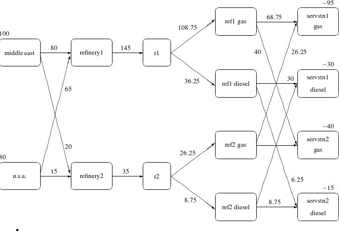
Notice that, in CONOUT=SOLUTION (Figure 6.7), the optimal flow through each arc in the network is given in the variable named _FLOW_, and the cost of flow through each arc is given in the variable _FCOST_.