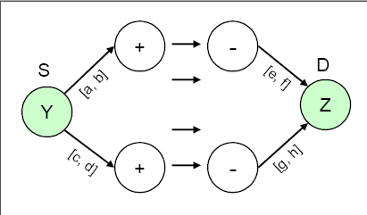
Consider the scenario depicted by Figure 6.31, where the supply and demand nodes have ranges; i.e., the amounts they can supply or demand are constrained to be within certain lower and upper bounds.

To model this situation, you first need to add a supply node with missing S supply value (the Y node in Figure 6.32) and a demand node with missing D demand value (the Z node in Figure 6.32). The bounds on the supply and demand nodes get transformed into upper/lower bounds on the arcs that connect them to nodes Y and Z, respectively. It might be necessary to have costs for these arcs to make it worthwhile for flow to traverse them, and subsequently to traverse the actual network. In practice, these costs represent procurement costs, profit from sales, etc.

You could set up all your network models in this fashion, not only in scenarios in which there are supply and demand ranges. For instance, this modeling technique could be used under the following conditions: