Example 6.14 Generalized Networks: Distribution Problem :: SAS/OR(R) 12.3 User's Guide: Mathematical Programming Legacy Procedures

Example 6.14 Generalized Networks: Distribution Problem

Consider a distribution problem (from Jensen and Bard 2003) with three supply plants ( – ) and five demand points ( – ). Further information about the problem is as follows:

: To be closed. Entire inventory must be shipped or sold to scrap. The scrap value is $5 per unit.
: Maximum production of 300 units with manufacturing cost of $10 per unit.
: The production in regular time amounts to 200 units and must be shipped. An additional 100 units can be produced using overtime at $14 per unit.
: Fixed demand of 200 units must be met.
: Contracted demand of 300 units. An additional 100 units can be sold at $20 per unit.
: Minimum demand of 200 units. An additional 100 units can be sold at $20 per unit. Additional units can be procured from at $4 per unit. There is a 5% “shipping loss” on the arc connecting these two nodes.
: Fixed demand of 150 units must be met.
: 100 units left over from previous shipments. No firm demand, but up to 250 units can be sold at $25 per unit.

Additionally, there is a 5% “shipping loss” on each of the arcs between supply and demand nodes.

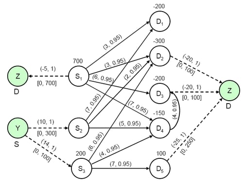
You can model this scenario as a generalized network. Since there are both fixed and varying supply and demand supdem values, you can transform this to a case where you need to address missing supply and demand simultaneously. As seen from Output 6.14.1, we have added two artificial nodes, Y and Z, with missing S supply value and missing D demand value, respectively. The extra production capability is depicted by arcs from node Y to the corresponding supply nodes, and the extra revenue generation capability of the demand points (and scrap revenue for ) is depicted by arcs to node Z.

Output 6.14.1: Distribution Problem

The following SAS data set has the complete information about the arc costs, multipliers, and node supdem values:

data dnodes;
   input _node_ $ _sd_ ;
   missing S D;
datalines;
S1   700
S2     0
S3   200
D1  -200
D2  -300
D3  -200
D4  -150
D5   100
Y      S
Z      D
;

data darcs;
   input _from_ $ _to_ $ _cost_ _capac_ _mult_;
datalines;
S1  D1    3   200  0.95
S1  D2    3   200  0.95
S1  D3    6   200  0.95
S1  D4    7   200  0.95
S2  D1    7   200  0.95
S2  D2    2   200  0.95
S2  D4    5   200  0.95
S3  D2    6   200  0.95
S3  D4    4   200  0.95
S3  D5    7   200  0.95
D4  D3    4   200  0.95
Y   S2   10   300  .
Y   S3   14   100  .
S1  Z   -5    700  .
D2  Z   -20   100  .
D3  Z   -20   100  .
D5  Z   -25   250  .
;

You can solve this problem by using the following call to PROC NETFLOW:

title1 'The NETFLOW Procedure';
proc netflow 
   nodedata = dnodes 
   arcdata  = darcs 
   conout   = dsol;
run;

The optimal solution is displayed in Output 6.14.2.

Output 6.14.2: Distribution Problem: Optimal Solution

The NETFLOW Procedure

Obs	_from_	_to_	_cost_	_capac_	_LO_	_mult_	_SUPPLY_	_DEMAND_	_FLOW_	_FCOST_
1	S1	D1	3	200	0	0.95	700	200	200.000	600.00
2	S2	D1	7	200	0	0.95	.	200	10.526	73.68
3	S1	D2	3	200	0	0.95	700	300	200.000	600.00
4	S2	D2	2	200	0	0.95	.	300	200.000	400.00
5	S3	D2	6	200	0	0.95	200	300	21.053	126.32
6	S1	D3	6	200	0	0.95	700	200	200.000	1200.00
7	D4	D3	4	200	0	0.95	.	200	10.526	42.11
8	S1	D4	7	200	0	0.95	700	150	100.000	700.00
9	S2	D4	5	200	0	0.95	.	150	47.922	239.61
10	S3	D4	4	200	0	0.95	200	150	21.053	84.21
11	S3	D5	7	200	0	0.95	200	.	157.895	1105.26
12	Y	S2	10	300	0	1.00	S	.	258.449	2584.49
13	Y	S3	14	100	0	1.00	S	.	0.000	0.00
14	S1	Z	-5	700	0	1.00	700	D	0.000	0.00
15	D2	Z	-20	100	0	1.00	.	D	100.000	-2000.00
16	D3	Z	-20	100	0	1.00	.	D	0.000	0.00
17	D5	Z	-25	250	0	1.00	100	D	250.000	-6250.00
										-494.32