Date and Time Intervals
Definition of a Date and Time Interval
An interval is a unit of measurement that SAS counts
within an elapsed period of time, such as days, months or hours. SAS
determines date and time intervals based on fixed points on the calendar
or clock. The starting point of an interval calculation defaults to
the beginning of the period in which the beginning value falls, which
might not be the actual beginning value that is specified. For example,
if you are using the INTCK function to count the months between two
dates, regardless of the actual day of the month that is specified
by the date in the beginning value, SAS treats the beginning value
as the first day of that month.
Interval Names and SAS Dates
Specific
interval names are used with SAS date values, while other interval
names are used with SAS time and datetime values. The interval names
that are used with SAS date values are YEAR, SEMIYEAR, QTR, MONTH,
SEMIMONTH, TENDAY, WEEK, WEEKDAY, and DAY. The interval names that
are used with SAS time and datetime values are HOUR, MINUTE, and SECOND.
Incrementing Dates and Times by Using Multipliers and by Shifting Intervals
SAS provides date, time,
and datetime intervals for counting different periods of elapsed time.
By using multipliers and shift indexes, you can create multiples of
intervals and shift their starting point to construct more complex
interval specifications.
Both the multiplier and
the shift–index arguments
are optional and default to 1. For example, YEAR, YEAR1, YEAR.1, and
YEAR1.1 are all equivalent ways of specifying ordinary calendar years
that begin in January. If you specify other values for multiplier and
for shift-index, you can create
multiple intervals that begin in different parts of the year. For
example, the interval WEEK6.11 specifies six-week intervals starting
on second Wednesdays.
For more information,
see Single-Unit Intervals in SAS Language Reference: Concepts, Multi-Unit Intervals in SAS Language Reference: Concepts, and Shifted Intervals in SAS Language Reference: Concepts.
Commonly Used Time Intervals
Time intervals that do
not nest within years or days are aligned relative to the SAS date
or datetime value 0. SAS uses the arbitrary reference time of midnight
on January 1, 1960, as the origin for non-shifted intervals. Shifted
intervals are defined relative to January 1, 1960.
For example, MONTH13
defines the intervals January 1, 1960, February 1, 1961, March 1,
1962, and so on, and the intervals December 1, 1958, November 1, 1957,
and so on, before the base date January 1, 1960.
As another example,
the interval specification WEEK6.13 defines six-week periods starting
on second Fridays. The convention of alignment relative to the period
that contains January 1, 1960, determines where to start counting
to determine which dates correspond to the second Fridays of six-week
intervals.
For a complete list
of the valid values for interval,
see Intervals Used with Date and Time Functions in SAS Language Reference: Concepts.
Retail Calendar Intervals: ISO 8601 Compliant
The retail industry
often accounts for its data by dividing the yearly calendar into four
13-week periods, based on one of the following formats: 4-4-5, 4-5-4,
or 5-4-4. The first, second, and third numbers specify the number
of weeks in the first, second, and third months of each period, respectively.
The intervals that are
created from the formats can be used in any of the following functions:
INTCINDEX, INTCK, INTCYCLE, INTFIT, INTFMT, INTGET, INTINDEX, INTNX,
INTSEAS, INTSHIFT, and INTTEST.
For more information,
see Retail Calendar Intervals: ISO 8601 Compliant in SAS Language Reference: Concepts.
Custom Time Intervals
Reasons for Using Custom Time Intervals
Standard time intervals (for example,
QTR, MONTH, WEEK, and so on) do not always fit the data. Additionally,
some time series are measured at standard intervals where there are
gaps in the data. For example, you might want to use fiscal months
that begin on the 10th day of each month. In this case, using the
MONTH interval is not appropriate because the MONTH interval begins
on the 1st day of each month. You can use a custom interval to model
data at a frequency that is familiar to the business and to eliminate
gaps in the data by compressing the data. The intervals must be listed
in ascending order. There cannot be gaps between intervals, and intervals
cannot overlap.
As another example,
you might want to collect data hourly for a business that is closed
at night. In this case, using the DTHOUR interval results in gaps
in the data that can cause problems in standard time series analysis.
You might also want to calculate the number of business days between
dates, excluding holidays and weekends, but holidays are counted when
you use the INTCK function with the WEEKDAY interval. These are cases
in which custom intervals can be used effectively.
Using Custom Time Intervals in a SAS Program
You can define custom
intervals in a data set within a SAS program. Using a custom interval
requires that you follow two steps for each interval:
-
Associate a data set name with a custom interval name by using the INTERVALDS= system option in an OPTIONS statement.Here is an example of the arguments in an INTERVALDS= system option. The example associates the data set StoreHoursDS with the custom interval StoreHours:
options intervalds=(StoreHours, StoreHoursDS);
For more information, see INTERVALDS= System Option in SAS System Options: Reference. -
The data set must contain the begin variable; it can also contain end and season variables. In your SAS program, include a FORMAT statement that is associated with the begin variable that specifies a SAS date, datetime, or numeric format that matches the begin variable data. If an end variable is present, include it in the FORMAT statement. A numeric format that is not a SAS date or SAS datetime format indicates that the values are observation numbers. If the end variable is not present, the implied value of end at each observation is one less than the value of begin at the next observation.
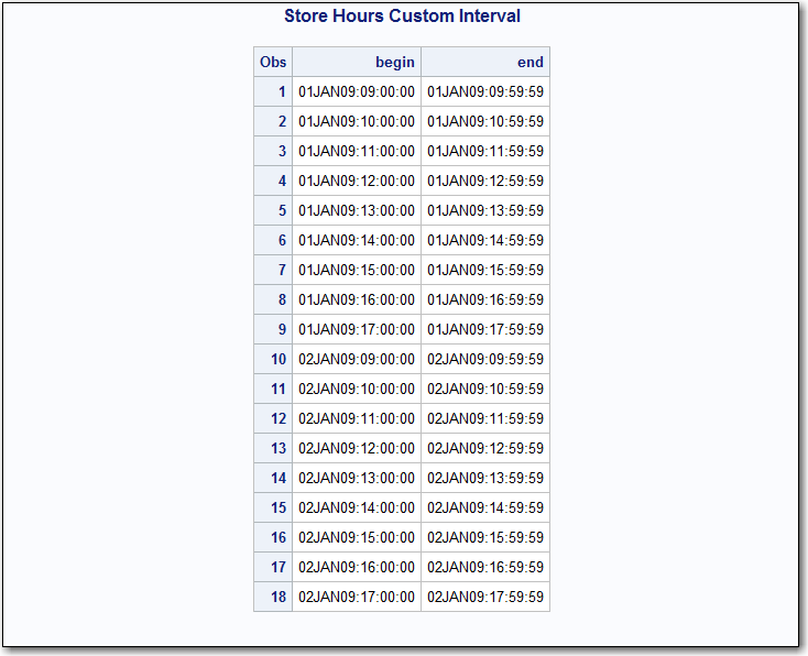
Example 1: Creating Store Hours for a Business Using the INTNX Function
The following DATA step
creates the StoreHoursDS data set for a business that is open from
9:00 AM to 6:00 PM Monday through Friday, and Saturday from 9:00 AM
to 1:00 PM. The example uses the INTNX Function, which increments a date, time, or
datetime value by a given time interval, and returns a date, time,
or datetime value. In this example, StoreHours is the interval, and
StoreHoursDS is the data set that contains user-supplied holidays:
options intervalds=(StoreHours=StoreHoursDS);
data StoreHoursDS(keep=begin end);
   start = '01JAN2009'd;
   stop  = '31DEC2009'd;
   do date = start to stop;
      dow = weekday(date);
      datetime=dhms(date,0,0,0);
      if dow not in (1,7) then
         do hour = 9 to 17;
            begin=intnx('hour',datetime,hour,'b');
            end=intnx('hour',datetime,hour,'e');
            output;
         end;
      else if dow = 7 then
         do hour = 9 to 12;
            begin=intnx('hour',datetime,hour,'b');
            end=intnx('hour',datetime,hour,'e');
            output;
         end;
   end;
   format begin end datetime.;
run;
title 'Store Hours Custom Interval';

proc print data=StoreHoursDS (obs=18);
run;
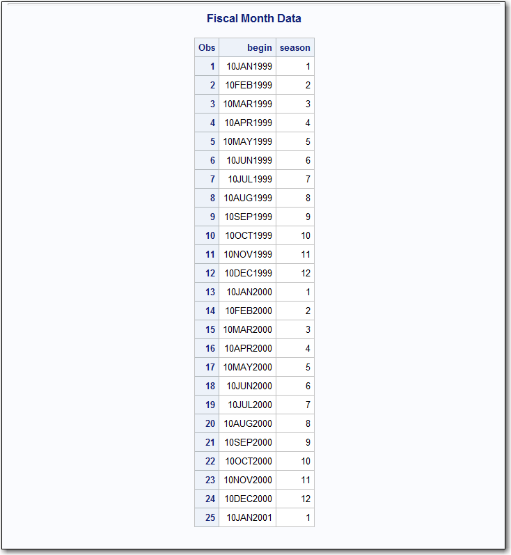
Example 2: Creating the Fiscal Month Custom Interval Using the INTNX Function
The following DATA step
creates the FMDS data set to define a custom interval, FiscalMonth,
which is appropriate for a business that uses fiscal months that start
on the 10th day of each month. The SAME alignment option of the INTNX
function specifies that the dates that are generated by the INTNX
function be the same day of the month as the date in the start variable.
The MONTH function assigns the month of the begin variable
to the season variable, which
specifies monthly seasonality:
options intervalds=(FiscalMonth=FMDS);
data FMDS(keep=begin season);
   start = '10JAN1999'd;
   stop  = '10JAN2001'd;
   nmonths = intck('month',start,stop);
   do i=0 to nmonths;
      begin = intnx('month',start,i,'S');
      season = month(begin);
      output;
   end;
   format begin date9.;
run;

proc print data=FMDS;
   title 'Fiscal Month Data';
run;
The difference between
the custom FiscalMonth interval and a standard interval is seen in
the following example. The output from the program compares how the
data is accumulated. For the FiscalMonth interval, values in the first
nine days of the month are accumulated with the interval that begins
in the previous month. For the standard MONTH interval, values in
the first nine days of the month are accumulated with the calendar
month.
data sales(keep=date sales);
   do date = '01JAN2000'd to '31DEC2000'd;
      month = MONTH(date);
      dayofmonth = DAY(date);
      sales = 0;
      if (dayofmonth lt 10) then sales= month/9;
      output;
   end;
   format date monyy.;
run;

proc timeseries data=sales out=dataInFiscalMonths;
   id date interval=FiscalMonth accumulate=total;
   var sales;
run;

proc timeseries data=sales out=dataInStdMonths;
   id date interval=Month accumulate=total;
   var sales;
run;

data compare;
   merge dataInFiscalMonths(rename=(sales=FM_sales))
         dataInStdMonths(rename=(sales=SM_sales));
   by date;
run;

title 'Standard Monthly Data and Fiscal Month Data';

proc print data=compare;
run;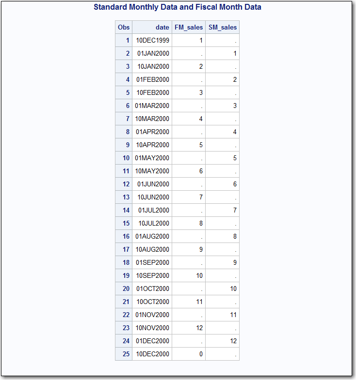
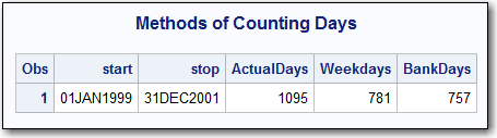
Example 3: Using Custom Intervals with the INTCK Function
The following example
uses custom intervals in the INTCK function to omit holidays when
counting business days:
options intervalds=(BankingDays=BankDayDS);
data BankDayDS(keep=begin);
   start = '15DEC1998'd;
   stop  = '15JAN2002'd;
   nwkdays = intck('weekday',start,stop);
   do i = 0 to nwkdays;
      begin = intnx('weekday',start,i);
      year = year(begin);
      if begin ne holiday('NEWYEAR',year) and
         begin ne holiday('MLK',year) and
         begin ne holiday('USPRESIDENTS',year) and
         begin ne holiday('MEMORIAL',year) and
         begin ne holiday('USINDEPENDENCE',year) and
         begin ne holiday('LABOR',year) and
         begin ne holiday('COLUMBUS',year) and
         begin ne holiday('VETERANS',year) and
         begin ne holiday('THANKSGIVING',year) and
         begin ne holiday('CHRISTMAS',year) then
      output;
   end;
   format begin date9.;
run;
data CountDays;
   start = '01JAN1999'd;
   stop  = '31DEC2001'd;
   ActualDays = intck('DAYS',start,stop);
   Weekdays   = intck('WEEKDAYS',start,stop);
   BankDays   = intck('BankingDays',start,stop);
   format start stop date9.;
run;

title 'Methods of Counting Days';

proc print data=CountDays;
run;
Best Practices for Custom Interval Names
The following items
list best practices to use when you are creating custom interval names:
-
Custom interval names should not conflict with existing SAS interval names. For example, if BASE is a SAS interval name, do not use the following formats for the name of a custom interval:
-
Calculations for custom intervals cannot be performed before the first begin value or after the last end value. If you use the begin variable only, then the last end value that you can calculate is the last begin value –1. If you forecast or backcast the time series, be sure to include time definitions for the forecast and backcast values.
-
CUSTBASEm.2 is never able to calculate a beginning period for the first date value in a data set because, by definition, the beginning of the first interval starts before the data set begins (at the – (m– 2) th observation). For example, you might have an interval called CUSTBASE4.2 with the first interval beginning before the first observation:
OBS -2 Start of partial CUSTBASE4.2 interval observation: -(4-2) = -2. -1 0 1 End of partial CUSTBASE4.2 interval observation: This is the first observation in the data set. 2 Start of first complete CUSTBASE4.2 interval. 3 4 5 End of first complete CUSTBASE4.2 interval. 6 Start of 2nd CUSTBASE4.2 interval. -
Include a variable named season in the custom interval data set to define the seasonal index. This result is similar to the result of
INTINDEX ('interval', date);In the following example, the data set is associated with the custom interval CUSTWEEK:Obs begin season 1 27DEC59 52 2 03JAN60 1 3 10JAN60 2 4 17JAN60 3 5 24JAN60 4 6 31JAN60 5
Copyright © SAS Institute Inc. All rights reserved.