Nonlinear Optimization Examples
Parameter Constraints
You can specify constraints in the following ways:
-
The matrix input argument "blc" enables you to specify boundary and general linear constraints.
-
The IML module input argument "nlc" enables you to specify general constraints, particularly nonlinear constraints.
Specifying the BLC Matrix
The input argument "blc" specifies an  constraint matrix, where
  is two more than the number of linear constraints, and
  is given by
![\[ n2 = \left\{ \begin{array}{ll} n & \mbox{if } 1 \leq n1 \leq 2 \\ n+2 & \mbox{if } n1 > 2 \end{array} \right. \]](images/imlug_nonlinearoptexpls0102.png)
The first two rows define lower and upper bounds for the n parameters, and the remaining  rows define general linear equality and inequality constraints. Missing values in the first row (lower bounds) substitute
for the largest negative floating point value, and missing values in the second row (upper bounds) substitute for the largest
positive floating point value. Columns
rows define general linear equality and inequality constraints. Missing values in the first row (lower bounds) substitute
for the largest negative floating point value, and missing values in the second row (upper bounds) substitute for the largest
positive floating point value. Columns  and
and  of the first two rows are not used.
The following c rows of the "blc" argument specify c linear equality or inequality constraints:
![\[ \sum _{j=1}^ n a_{ij} x_ j \quad (\leq | = | \geq ) \quad b_ i , \quad i=1,\ldots ,c \]](images/imlug_nonlinearoptexpls0106.png)
Each of these c rows contains the coefficients  in the first n columns. Column specifies the kind of constraint, as follows:
-
blc
![$[n+1]= 0$](images/imlug_nonlinearoptexpls0108.png) indicates an equality constraint.
indicates an equality constraint.
-
blc
![$[n+1]= 1$](images/imlug_nonlinearoptexpls0109.png) indicates a
indicates a  inequality constraint.
-
blc
![$[n+1]= -1$](images/imlug_nonlinearoptexpls0111.png) indicates a
indicates a  inequality constraint.
Column specifies the right-hand side,  . A missing value in any of these rows corresponds to a value of zero.
For example, suppose you have a problem with the following constraints on  ,
, ,
,  ,
,  :
:
![\[ \begin{array}{rcccr} 2 & \le & x_1 & \le & 100 \\ & & x_2 & \le & 40 \\ 0 & \le & x_4 & \\[0.2in]\end{array} \]](images/imlug_nonlinearoptexpls0118.png)
![\[ \begin{array}{rcrcrcrcl} 4x_1 & + & 3x_2 & - & x_3 & & & \le & 30 \\ & & x_2 & & & + & 6x_4 & \ge & 17 \\ x_1 & - & x_2 & & & & & = & 8 \\ \end{array} \]](images/imlug_nonlinearoptexpls0119.png)
The following statements specify the matrix CON, which can be used as the "blc" argument to specify the preceding constraints:
proc iml;
con = {   2   .   .   0    .    . ,
        100  40   .   .    .    . ,
          4   3  -1   .   -1   30 ,
          .   1   .   6    1   17 ,
          1  -1   .   .    0    8 };
Specifying the NLC and JACNLC Modules
The input argument "nlc" specifies an IML module that returns a vector, c, of length  , with the values,
  , of the linear or nonlinear constraints
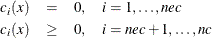
for a given input parameter point x.
Note: You must specify the number of equality constraints,  , and the total number of constraints, , returned by the "nlc" module to allocate memory for the return vector. You can do this with the opt[11] and opt[10] arguments, respectively.
For example, consider the problem of minimizing the objective function  in the interior of the unit circle,
  . The constraint can also be written as
 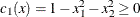 . The following statements specify modules for the objective and constraint functions and call the NLPNMS subroutine to solve
the minimization problem:
. The following statements specify modules for the objective and constraint functions and call the NLPNMS subroutine to solve
the minimization problem:
proc iml;
start F_UC2D(x);
   f = x[1] * x[2];
   return(f);
finish F_UC2D;

start C_UC2D(x);
   c = 1. - x * x`;
   return(c);
finish C_UC2D;

x = j(1,2,1.);
optn= j(1,10,.); optn[2]= 3; optn[10]= 1;
CALL NLPNMS(rc,xres,"F_UC2D",x,optn) nlc="C_UC2D";
To avoid typing multiple commas, you can specify the "nlc" input argument with a keyword, as in the preceding code. The number of elements of the return vector is specified by OPTN![$[10]=1$](images/imlug_nonlinearoptexpls0125.png) . There is a missing value in OPTN
. There is a missing value in OPTN![$[11]$](images/imlug_nonlinearoptexpls0126.png) , so the subroutine assumes there are zero equality constraints.
, so the subroutine assumes there are zero equality constraints.
The NLPQN algorithm uses the  Jacobian matrix of first-order derivatives
![\[ ( \nabla _ x c_ i(x) ) = \left( \frac{\partial c_ i}{\partial x_ j} \right) , \quad i= 1,\ldots ,nc, \quad j=1,\ldots ,n \]](images/imlug_nonlinearoptexpls0127.png)
of the equality and inequality constraints, , for each point passed during the iteration. You can use the "jacnlc" argument to specify an IML module that returns the Jacobian matrix JC. If you specify the "nlc" module without using the "jacnlc" argument, the subroutine uses finite-difference approximations of the first-order derivatives of the constraints.
Note: The COBYLA algorithm in the NLPNMS subroutine and the NLPQN subroutine are the only optimization techniques that enable you to specify nonlinear constraints with the "nlc" input argument.