Nonlinear Optimization Examples
Rosen-Suzuki Problem
The Rosen-Suzuki problem is a function of four variables with three nonlinear constraints on the variables. It is taken from problem 43 of Hock and Schittkowski (1981). The objective function is

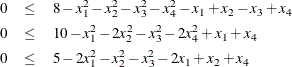
The nonlinear constraints are
Since this problem has nonlinear constraints, only the NLPQN and NLPNMS subroutines are available to perform the optimization. The following code solves the problem with the NLPQN subroutine:
proc iml;
start F_HS43(x);
   f = x*x` + x[3]*x[3] - 5*(x[1] + x[2]) - 21*x[3] + 7*x[4];
   return(f);
finish F_HS43;
start C_HS43(x);
   c = j(3,1,0.);
   c[1] = 8 - x*x` - x[1] + x[2] - x[3] + x[4];
   c[2] = 10 - x*x` - x[2]*x[2] - x[4]*x[4] + x[1] + x[4];
   c[3] = 5 - 2.*x[1]*x[1] - x[2]*x[2] - x[3]*x[3]
            - 2.*x[1] + x[2] + x[4];
   return(c);
finish C_HS43;
x = j(1,4,1);
optn= j(1,11,.); optn[2]= 3; optn[10]= 3; optn[11]=0;
ods select ProblemDescription IterStart IterHist IterStop ParameterEstimates;
call nlpqn(rc,xres,"F_HS43",x,optn) nlc="C_HS43";
The F_HS43 module specifies the objective function, and the C_HS43 module specifies the nonlinear constraints. The OPTN vector is passed to the subroutine as the OPT input argument. See the section Options Vector for more information. The value of OPTN[10] represents the total number of nonlinear constraints, and the value of OPTN[11] represents the number of equality constraints. In the preceding code, OPTN[10]=3 and OPTN[11]=0, which indicate that there are three constraints, all of which are inequality constraints. In the subroutine calls, instead of separating missing input arguments with commas, you can specify optional arguments with keywords, as in the CALL NLPQN statement in the preceding code. For details about the CALL NLPQN statement, see the section NLPQN Call.
The initial point for the optimization procedure is  , and the optimal point is
 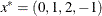 , with an optimal function value of
  . Part of the output produced is shown in Figure 15.4.
Figure 15.4: Solution to the Rosen-Suzuki Problem by the NLPQN Subroutine
| Iteration | Restarts | Function Calls |
Objective Function |
Maximum Constraint Violation |
Predicted Function Reduction |
Step Size |
Maximum Gradient Element of the Lagrange Function |
|
|---|---|---|---|---|---|---|---|---|
| 1 | 0 | 2 | -41.88007 | 1.8988 | 13.6803 | 1.000 | 5.647 | |
| 2 | 0 | 3 | -48.83264 | 3.0280 | 9.5464 | 1.000 | 5.041 | |
| 3 | 0 | 4 | -45.33515 | 0.5452 | 2.6179 | 1.000 | 1.061 | |
| 4 | 0 | 5 | -44.08667 | 0.0427 | 0.1732 | 1.000 | 0.0297 | |
| 5 | 0 | 6 | -44.00011 | 0.000099 | 0.000218 | 1.000 | 0.00906 | |
| 6 | 0 | 7 | -44.00001 | 2.573E-6 | 0.000014 | 1.000 | 0.00219 | |
| 7 | 0 | 8 | -44.00000 | 9.118E-8 | 5.097E-7 | 1.000 | 0.00022 |
| Optimization Results | |||
|---|---|---|---|
| Iterations | 7 | Function Calls | 9 |
| Gradient Calls | 9 | Active Constraints | 2 |
| Objective Function | -44.00000026 | Maximum Constraint Violation | 9.1176306E-8 |
| Maximum Projected Gradient | 0.0002265341 | Value Lagrange Function | -44 |
| Maximum Gradient of the Lagran Func | 0.00022158 | Slope of Search Direction | -5.097332E-7 |
In addition to the standard iteration history, the NLPQN subroutine includes the following information for problems with nonlinear constraints:
-
CONMAX is the maximum value of all constraint violations.
-
PRED is the value of the predicted function reduction used with the GTOL and FTOL2 termination criteria.
-
ALFA is the step size
 of the quasi-Newton step.
-
LFGMAX is the maximum element of the gradient of the Lagrange function.