Statistical Graphics

Histograms

You can use the HISTOGRAM subroutine to create a histogram. The required argument is a vector that contains values of a continuous variable.

The following statements read the MPG_City variable from the Sashelp.Cars data set:

proc iml;
use Sashelp.Cars;
read all var {MPG_City};
close Sashelp.Cars;

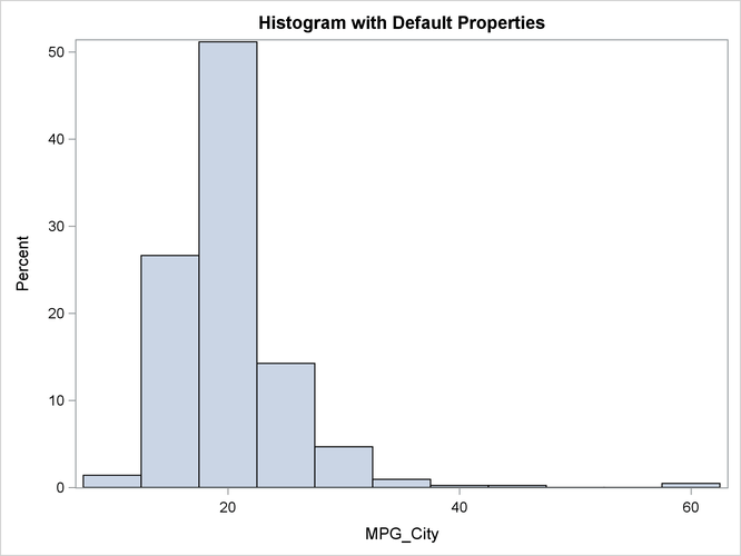
The following statements create a simple histogram, which is shown in Figure 16.6:

title "Histogram with Default Properties";
call Histogram(MPG_City);

Figure 16.6: Histogram with Default Options

For a more complicated example, the following statements create a histogram by using the SCALE=, DENSITY=, REBIN=, GRID=, LABEL=, and XVALUES= options: The result is shown in Figure 16.7.

title "Histogram with Density Curves";
call Histogram(MPG_City)
          scale="Percent"
          density={"Normal" "Kernel"}
          rebin={0 5}
          grid="y"
          label="Miles per Gallon (City)"
          xvalues=do(0, 60, 10);

Figure 16.7: Histogram with Overlaid Densities

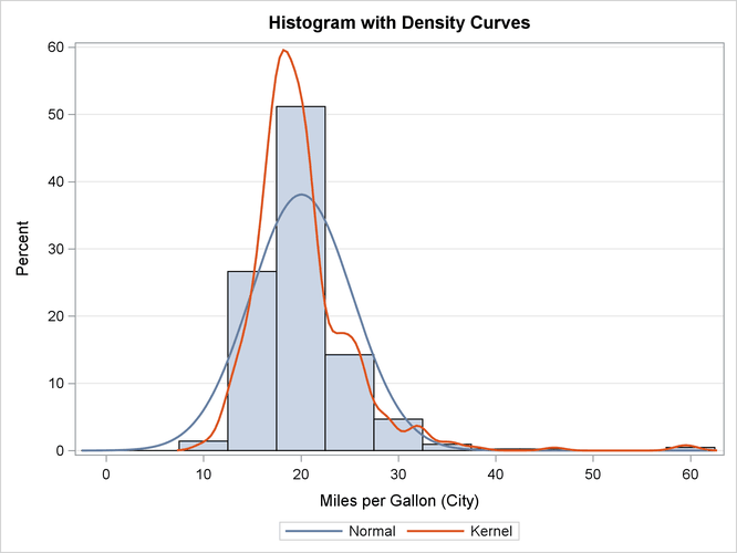
The following list explains the options that are used to create Figure 16.7:

The SCALE= option specifies the scaling that is applied to the vertical axis of the histogram. In Figure 16.6, the vertical axis is scaled to represent the percentage of observations in each bar.
The DENSITY= option specifies whether to overlay a density estimate on the histogram. In Figure 16.6, a normal density estimate and a kernel density estimate are overlaid.
The REBIN= option specifies two numerical values that set the location of the first bins and the width of bins. In Figure 16.6, the bins are anchored at the value 0 and have a width of 5 units.
The GRID= option specifies whether grid lines are displayed for the X and Y axes. Figure 16.6 shows grid lines for the Y axis.
The LABEL= option specifies axis labels. In Figure 16.6, a label is specified for the X axis.
The XVALUES= option specifies a vector of values for ticks for the X and Y axes. In Figure 16.6, tick marks are placed every 10 units in the interval $[0,60]$ .