General Statistics Examples

You can solve the following general linear programming problem by using the LPSOLVE call :

Consider the following product mix example (Hadley 1962). A shop that has three machines, A, B, and C, turns out four different products. Each product must be processed on each of the three machines (for example, lathes, drills, and milling machines). The following table shows the number of hours required by each product on each machine:

The weekly time available on each of the machines is 2,000, 8,000, and 5,000 hours, respectively. The products contribute 5.24, 7.30, 8.34, and 4.18 to profit, respectively. What mixture of products can be manufactured to maximize profit?

The following SAS/IML program calls the LPSOLVE routine and displays a summary of the optimization results:

proc iml;
names={'product 1' 'product 2' 'product 3' 'product 4'};
/* coefficients of the linear objective function             */
c = {5.24 7.30 8.34 4.18};
/* coefficients of the constraint equation                   */
A = { 1.5  1  2.4  1   ,
      1    5  1    3.5 ,
      1.5  3  3.5  1   };

/* right-hand side of constraint equation                    */
b = { 2000, 8000, 5000};
/* operators: 'L' for <=, 'G' for >=, 'E' for =              */
ops = { 'L', 'L', 'L' };

n=ncol(A);                            /* number of variables */
cntl = j(1,7,.);                           /* control vector */
cntl[1] = -1;               /* 1 for minimum; -1 for maximum */
call lpsolve(rc, value, x, dual, redcost,
             c, A, b, cntl, ops);

print x[r=names L='Optimal Product Mix'];
print value[L='Maximum Profit'];
lhs = A*x;
Constraints = lhs || b;
print Constraints[r={"Machine1" "Machine2" "Machine3"}
                  c={"Actual" "Upper Bound"}
                  L="Time Constraints"];

The results from this example are shown in Output 10.9.1. The optimal mix of products is to produce 295 units of product 1, 1,500 units of product 2, no units of product 3, and 58 units of product 4. Manufacturing that product mix results in an optimal profit and also utilizes the maximum availability of the three machines.

The next example shows how to find the minimum cost flow through a network by using linear programming. The network consists of five nodes, named A, B, C, D, and E. Seven arcs connect certain nodes. The arcs are named by the tail and head nodes that define the arc. Figure 10.1 shows the network.

Figure 10.1: A Network of Nodes and Arcs

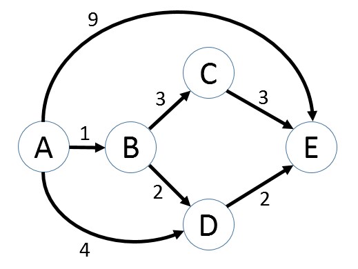
Suppose that some nodes have an excess supply of goods whereas others have a deficit of goods, and suppose that you want to transport goods from the nodes that have excess supply to nodes that have the demand. Each route (arc) between nodes has a cost that is associated with it. In Figure 10.1, the cost is represented by a number next to an arc. Given a distribution of goods, what is the optimal way to move goods through the network?

This example sets up the problem and calls the LPSOLVE subroutine to find an optimal solution. In the example, two units of goods are located at node A. One unit needs to be moved to node D; the other unit needs to travel to node E.

The first part of the problem requires generating the node-arc incidence matrix.

arcs = { 'ab' 'bd' 'ad' 'bc' 'ce' 'de' 'ae' }; /* decision variables  */
n=ncol(arcs);                                  /* number of variables */
nodes = {'a', 'b', 'c', 'd', 'e'};
inode = substr(arcs, 1, 1);
onode = substr(arcs, 2, 1);
/* coefficients of the constraint equation */
A = j(nrow(nodes), n, 0);
do j = 1 to n;
   A[,j] = (inode[j]=nodes) - (onode[j]=nodes);
end;

The matrix A constrains the goods to flow through the existing arcs between nodes. A solution to the problem is a vector that contains the number of goods that flow through each arc. The cost of moving goods is a linear function of a solution. The following statements define the supply and demand of goods within the network and call the LPSOLVE subroutine to obtain a solution that minimizes the cost:

/* coefficients of the linear objective function             */
cost = { 1 2 4 3 3 2 9 };
/* right-hand side of constraint equation                    */
supply = { 2, 0, 0, -1, -1 };
/* operators: 'L' for <=, 'G' for >=, 'E' for =              */
ops = repeat('E',nrow(nodes),1);

cntl = j(1,7,.);                           /* control vector */
cntl[1] = 1;                /* 1 for minimum; -1 for maximum */
call lpsolve(rc, value, x, dual, redcost,
             cost, A, supply, cntl, ops);

print value[L='Minimum Cost'];
print x[r=arcs L='Optimal Flow'];

The solution is shown in Output 10.9.2. The optimal solution is to move both units along arc AB and then along arc BD. One unit stays at node D, while the other proceeds along arc DE. The minimum cost is 8.