Robust Regression Examples
This section creates graphs that illustrate the results of the MVE and MCD procedures. The following statements load the RobustMC.sas program, which is included in the SAS/IML sample library. The LOAD MODULES=_ALL_ statement loads modules that are defined
in the program. In particular, this section uses the MVESCATTER and MCDSCATTER modules.
%include "C:\<path>\RobustMC.sas";
proc iml;
load module=_all_;
Jerison (1973) reported data for the body mass (in kilograms) and brain mass (in grams) of ![]() animals. These data were further analyzed in Rousseeuw and Leroy (1987). Instead of the original data, the following example uses the logarithms of the measurements of the two variables:
animals. These data were further analyzed in Rousseeuw and Leroy (1987). Instead of the original data, the following example uses the logarithms of the measurements of the two variables:
/* Log(Body Mass) Log(Brain Mass) */
mass={ 0.1303338  0.9084851,  2.6674530  2.6263400,
       1.5602650  2.0773680,  1.4418520  2.0606980,
       0.0170333  0.7403627,  4.0681860  1.6989700,
       3.4060290  3.6630410,  2.2720740  2.6222140,
       2.7168380  2.8162410,  1.0000000  2.0606980,
       0.5185139  1.4082400,  2.7234560  2.8325090,
       2.3159700  2.6085260,  1.7923920  3.1205740,
       3.8230830  3.7567880,  3.9731280  1.8450980,
       0.8325089  2.2528530,  1.5440680  1.7481880,
      -0.9208187  0.0000000, -1.6382720 -0.3979400,
       0.3979400  1.0827850,  1.7442930  2.2430380,
       2.0000000  2.1959000,  1.7173380  2.6434530,
       4.9395190  2.1889280, -0.5528420  0.2787536,
      -0.9136401  0.4771213,  2.2833010  2.2552720};
By default, the MVE subroutine uses randomly selected subsets rather than all subsets. The following statements specify that all 3,276 subsets of three observations out of 28 observations be generated and evaluated. Output 12.4.1 shows partial results of the analysis.
optn = j(5,1,.);
optn[1] = 1;             /* print basic output */
optn[2] = 1;             /* print covariance matrices */
optn[5]= -1;             /* nrep: use all subsets */

ods exclude EigenRobust Distances DistrRes;
call mve(sc, xmve, dist, optn, mass);
ods select all;
Output 12.4.1: Results of MVE Robust Estimation
| There are 3276 subsets of 3 cases out of 28 cases. |
| All 3276 subsets will be considered. |
| Complete Enumeration for MVE |
| 25 % of calculations have been executed. |
| 75 % of calculations have been executed. |
| Minimum Criterion= 0.439709106 |
| Among 3276 subsets 0 are singular. |
| Initial MVE Location Estimates |
|
|---|---|
| VAR1 | 1.3859759333 |
| VAR2 | 1.8022650333 |
| Distribution of Robust Distances |
| Cutoff Value = 2.7162030315 |
| The cutoff value is the square root of the 0.975 quantile of the chi square distribution with 2 degrees of freedom. |
| There are 5 points with large robust distances receiving zero weights. These may include boundary cases. Only points whose robust distances are substantially larger than the cutoff value should be considered outliers. |
The MVE routine also returns information in the sc, xmve, and dist matrices. The following statements print some of that information:
r1 = {"Quantile", "Number of Subsets", "Number of Singular Subsets",
      "Number of Nonzero Weights", "Min Objective Function",
      "Min Distance", "Chi-Square Cutoff Value"};
RobustCenter = xmve[1,];
RobustCov =    xmve[3:4,];
print sc[r=r1],
      RobustCenter[c={"X1","X2"}],
      RobustCov[r={"X1","X2"} c={"X1","X2"}];
MVEOutliers = loc(dist[3,]=0);
print MVEOutliers;
The first table in Output 12.4.2 shows some summary statistics about the combinatoric optimization (complete subset sampling) during the MVE algorithm. The algorithm considers subsets of three observations and strives to find the subset that minimizes the volume of an ellisoid that contains 15 points. The MVE algorithm considers 3,276 subsets, of which zero are singular. The minimum volume is found to be 1.47.
The mean vector is contained in the RobustCenter vector. The covariance matrix is contained in the RobustCov matrix.
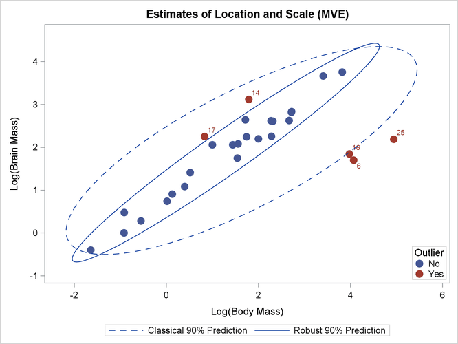
Based on that center and covariance matrix, a Mahalanobis-type distance (called the robust distance) that measures each observation’s distance from the robust center is computed. Observations that are more than a certain distance (the "Cutoff Value") from the center are classified as outliers. For these data, observations 6, 14, 16, 17, and 25 are classified as outliers.
You can call the MVESCATTER subroutine, which is included in the sample library in the file RobustMC.sas, to plot the classical and robust confidence ellipsoids, as follows:
optn = j(5,1,.); optn[5]= -1;
vnam = {"Log(Body Mass)","Log(Brain Mass)"};
titl = "Estimates of Location and Scale (MVE)";
call MVEScatter(mass, optn, 0.9, vnam, titl);
The plot is shown in Output 12.4.3.
MCD is another subroutine that can be used to compute the robust location and the robust covariance of multivariate data sets. The following statements call the MCD subroutine and produce Output 12.4.4
/* MCD: Use Random Subsets */
optn = j(5,1,.);
call mcd(sc, xmve, dist, optn, mass);

r1 = {"Quantile", "Number of Subsets", "Number of Singular Subsets",
      "Number of Nonzero Weights", "Min Objective Function",
      "Min Distance", "Chi-Square Cutoff Value"};
RobustCenter = xmve[1,];
RobustCov =    xmve[3:4,];
print sc[r=r1],
      RobustCenter[c={"X1","X2"}],
      RobustCov[r={"X1","X2"} c={"X1","X2"}];
The results are similar to Output 12.4.1. For the MCD subroutine, 500 random subsets are used for the optimization. The robust center and covariance matrices are slightly different from those found by the MVE subroutine. However, the observations that are classified as outliers (not shown) are the same.
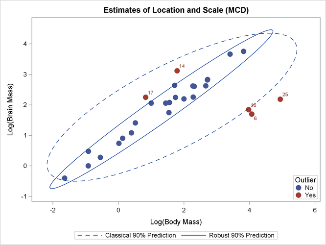
You can call the MCDSCATTER subroutine, which is included in the SAS/IML sample library, to plot the classical and robust confidence ellipsoids, as follows:
optn = j(5,1,.); optn[5]= -1;
vnam = { "Log(Body Mass)","Log(Brain Mass)" };
titl = "Estimates of Location and Scale (MCD)";
call MCDScatter(mass, optn, 0.9, vnam, titl);
The plot is shown in Output 12.4.5. It looks very similar to Output 12.4.3.