TPSPLNEV Call :: SAS/IML(R) 13.1 User's Guide

TPSPLNEV Call

CALL TPSPLNEV (pred, xpred, x, coeff) ;

The TPSPLNEV subroutine evaluates the thin-plate smoothing spline (TPSS) at new data points. It is used after the TPSPLINE subroutine fits a thin-plate spline model to data.

The TPSPLNEV subroutine returns the following value:

pred: is an $m \times 1$ vector of the predicated values of the TPSS fit evaluated at $m$ new data points.

The input arguments to the TPSPLNEV subroutine are as follows:

xpred: is an $m \times k$ matrix of data points at which the $f_\lambda$ is evaluated, where $m$ is the number of new data points and $k$ is the number of variables in the spline model.
x: is an $n \times k$ matrix of design points that is used as an input of TPSPLINE call.
coeff: is the coefficient vector returned from the TPSPLINE call.

See the previous section on the TPSPLINE call for details about the TSPLNEV subroutine.

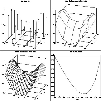
The following example contains two independent variables and one response variable. The first panel of Figure 24.410 shows a plot of the data. The following statements define the data and a sequence of $\lambda$ values within the interval $(-3.8, -3.3)$ . The TPSPLINE call fits the thin-plate smoothing spline on those design points and computes the GCV function for each value of $\lambda$ within the interval.

x={ -1.0 -1.0,    -1.0 -1.0,    -0.5 -1.0,    -0.5 -1.0,
     0.0 -1.0,     0.0 -1.0,     0.5 -1.0,     0.5 -1.0,
     1.0 -1.0,     1.0 -1.0,    -1.0 -0.5,    -1.0 -0.5,
    -0.5 -0.5,    -0.5 -0.5,     0.0 -0.5,     0.0 -0.5,
     0.5 -0.5,     0.5 -0.5,     1.0 -0.5,     1.0 -0.5,
    -1.0  0.0,    -1.0  0.0,    -0.5  0.0,    -0.5  0.0,
     0.0  0.0,     0.0  0.0,     0.5  0.0,     0.5  0.0,
     1.0  0.0,     1.0  0.0,    -1.0  0.5,    -1.0  0.5,
    -0.5  0.5,    -0.5  0.5,     0.0  0.5,     0.0  0.5,
     0.5  0.5,     0.5  0.5,     1.0  0.5,     1.0  0.5,
    -1.0  1.0,    -1.0  1.0,    -0.5  1.0,    -0.5  1.0,
     0.0  1.0,     0.0  1.0,     0.5  1.0,     0.5  1.0,
     1.0  1.0,     1.0  1.0 };

y = {15.54, 15.76, 18.67, 18.50, 19.66, 19.80, 18.60, 18.52,
     15.87, 16.04, 10.92, 11.14, 14.81, 14.83, 16.56, 16.44,
     14.91, 15.06, 10.92, 10.94,  9.61,  9.65, 14.03, 14.03,
     15.77, 16.00, 14.00, 14.03,  9.56,  9.58, 11.21, 11.09,
     14.84, 14.99, 16.55, 16.51, 14.98, 14.72, 11.15, 11.17,
     15.83, 15.96, 18.64, 18.56, 19.54, 19.81, 18.57, 18.61,
     15.87, 15.90 };

lambda = T( do(-3.8, -3.3, 0.1) );
call tpspline(fit, coef, adiag, gcv, x, y, lambda);

Figure 24.409: Output from the TPSPLINE Subroutine

SUMMARY OF TPSPLINE CALL

Summary of Tpspline Call
Number of Observations	50
Number of Unique Design Points	25
Dimension of Polynomial Space	3
Number of Parameters	28
GCV Estimate of Lambda	6.6006258E-6
Smoothing Penalty	2558.7692018
Residual Sum of Squares	0.2434454154
Trace of (I-A)	25.402044412
Sigma^2 Estimate	0.0095836938
Sum of Squares for Replication	0.23965

The TPSPLINE call returns the fitted values at each design point. The fitted surface is plotted in the second panel of Figure 24.410. The fourth panel shows a plot of the GCV function values against lambda.

You can use the TPSPLNEV call to score the thin-plate spline at a new set of points. The following statements generate a dense grid on $[-1,1] \times [-1,1]$ . The x and coef matrices are used to evaluate the thin-plate spline on the new grid of points:

xGrid = T( do(-1, 1, 0.1) );
yGrid = T( do(-1, 1, 0.1) );
do i = 1 to nrow(xGrid);
   x1 = x1 // repeat(xGrid[i], nrow(yGrid));
   x2 = x2 // yGrid;
end;
xpred = x1 || x2;

call tpsplnev(pred, xpred, x, coef);

The third panel of Figure 24.410 shows the thin-plat spline evaluated on the grid of points.

Figure 24.410: Plots of Fitted Surface