LPSOLVE Call :: SAS/IML(R) 13.1 User's Guide

LPSOLVE Call

CALL LPSOLVE (rc, objvalue, x, dual, reducost, c, a, b <*>, cntl <*>, rowsense <*>, range <*>, l <*>, u ) ;

The LPSOLVE subroutine solves a linear programming problem. It uses a different input format and solver options from the LP call and is the preferred method for solving linear programming problems.

The input arguments to the LPSOLVE subroutine are as follows:

c

is a vector of dimension $n$ of objective function coefficients. A missing value is treated as 0.

a

is an $m \times n$ matrix of the technological coefficients. A missing value is treated as 0.

b

is a vector of dimension $m$ of constraints’ right-hand sides (RHS). For a range constraint, b is its constraint upper bound. A missing value is treated as 0.

cntl

is an optional vector that contains one to eight elements that represent the LPSOLVE subroutine’s control options. The default value is used if an option is not specified or its value is a missing value. If cntl=(objsense, printlevel, maxtime, maxiter, presolve, algorithm,scaling, tol), then

objsense: specifies whether it is a minimization or a maximization problem, where 1 specifies minimization and $-1$ specifies maximization. The default value is 1.
printlevel: specifies the type of messages printed to the log. A value of 0 prints warning and error messages only, whereas 1 prints solution information in addition to warning and error messages. The default value is 0.
maxtime: specifies an upper bound of running time in seconds. The default value is effectively unbounded.
maxiter: specifies the maximum number of iterations to be processed. The default value is effectively unbounded.
presolve: specifies the presolve option, where 0 indicates no presolve and 1 indicates an automatic presolve option.The default value is 1.
algorithm: specifies the type of solver, where 1 specifies primal simplex, 2 specifies dual simplex, and 3 specifies interior point algorithm. The default value is 2.
scaling: specifies whether to scale the problem matrix, where 0 turns off scaling and 1 turns on scaling. The default value is 1.
tol: specifies a feasibility and optimality tolerance. The default value is $10^{-6}$ .

rowsense

is an optional row vector of dimension $m$ that specifies the sense of each constraint. The values can be E, L, G, or R for equal, less than or equal to, greater than or equal to, or range constraint. If this vector is missing, the solver treats the constraints as E type constraints.

range

is an optional row vector of dimension $m$ that specifies the range of the constraints. The row sense for a range constraint is R. For the non-range constraints, the corresponding values are ignored. For a range constraint, the range value is the difference between its constraint lower bound and its constraint upper bound b, so it must be nonnegative.

l

is an optional column vector of dimension $n$ that specifies lower bounds on the decision variables. If you do not specify l or l[j] has a missing value, then the lower bound of variable $j$ is assumed to be 0.

u

is an optional column vector of dimension $n$ that specifies upper bounds on the decision variables. If you do not specify u or u[j] has a missing value, the upper bound of variable $j$ is assumed to be infinity.

The LPSOLVE subroutine returns the following values:

rc

returns one of the following scalar return codes:

rc	Termination Reason
0	The solution is optimal.
1	The time limit was exceeded.
2	The maximum number of iterations was exceeded.
3	The solution is infeasible.
4	The solution is unbounded or infeasible.
5	The subroutine could not obtain enough memory.
6	The subroutine failed to solve the problem.

objvalue

returns the optimal or final objective value at termination.

x

returns the current primal solution in a column vector of length $n$ .

dual

returns the current dual solution in a row vector of length $m$ .

reducost

returns reduced cost in a column vector of length $n$ .

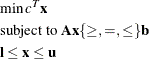
The LPSOLVE subroutine solves linear programs. A standard linear program has the following formulation:

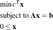
$\begin{eqnarray*} & & \min c^{T}\mb {x} \\ & & \mbox{subject to } \mb {Ax} \{ \geq ,=,\leq \} \mb {b} \\ & & \mb {l} \leq \mb {x} \leq \mb {u} \end{eqnarray*}$

If only $c$ , $\mb {A}$ , and $\mb {b}$ are present, then LPSOLVE solves the following linear programming problem by default:

$\begin{eqnarray*} & & \min c^{T}\mb {x} \\ & & \mbox{subject to } \mb {Ax} = \mb {b} \\ & & 0 \leq \mb {x} \end{eqnarray*}$

The primal and dual simplex solvers implement the two-phase simplex method. In phase I, the solver tries to find a feasible solution. If it does not find a feasible solution the LP is infeasible; otherwise, the solver enters phase II to solve the original LP. The interior point solver implements a primal-dual predictor-corrector interior point algorithm.

Consider the following example:

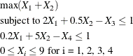
$\begin{eqnarray*} & & \max ( X_1 + X_2 ) \\ & & \mbox{subject to } 2X_1 + 0.5X_2 -X_3 \leq 1 \\ & & 0.2X_1 + 5X_2 -X_4 \leq 1 \\ & & 0 \leq X_ i \leq 9 \mbox{ for i = 1, 2, 3, 4} \end{eqnarray*}$

The problem is solved by using the following statements:

object = {  1   1   0   0 };
coef   = {  2  .5  -1   0,
           .2   5   0  -1};
b =      { 1,   1 };
l = { 0 0 0 0 };
u = { 9 9 9 9 };
rowsense = {'L','L'};
cntl= -1;
call lpsolve (rc,objv,x,dual,rd,object,coef,b,cntl,rowsense,,l,u);
print objv, x, dual, rd;

Figure 24.199: Example LPSOLVE Call

objv
6.3636364

x
4.5454545
1.8181818
9
9

dual
0.4848485	0.1515152

rd
0
0
0.4848485
0.1515152